Full-Text Search (BM25)
This document explains how Lattice's full-text search works, from text input to ranked results.
Overview
Full-text search allows you to find documents containing specific words or phrases, ranked by relevance. Lattice implements the BM25 (Best Match 25) ranking algorithm, the same algorithm used by Elasticsearch and other production search engines.
An index covers exactly one label and one property — Document.body, say. You
declare it once, and writing that property keeps it current. Sections 13 to 16
cover how a declaration is stored, how one set of trees carries many indexes, how
writes maintain them, and why the one-label-one-property shape is what lets a
query read the index instead of scanning.
The FTS system consists of five components:

1. Tokenizer
The tokenizer breaks text into searchable tokens.
What It Does
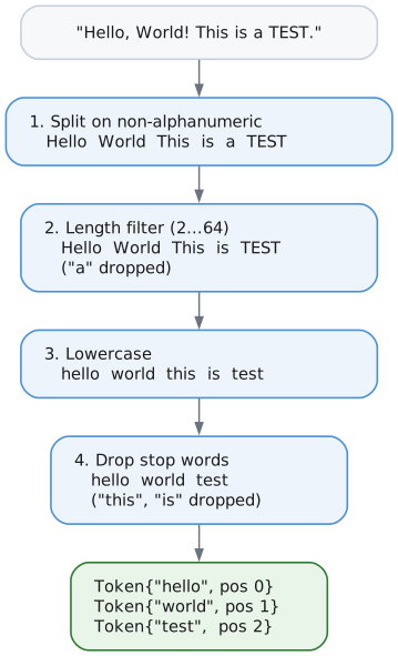
Given input text:
"The quick brown fox jumps over the lazy dog"
The tokenizer produces:
["quick", "brown", "fox", "jumps", "lazy", "dog"]
Notice "The", "the", and "over" are missing—they're stop words.
How It Works
Stop Words
Stop words are common words that add little search value. Lattice supports stop word filtering for 11 languages:
| Language | Example Stop Words |
|---|---|
| English | the, and, is, a, to, of, in, that, it |
| German | der, die, das, und, ist, in, zu, den |
| French | le, la, les, de, et, en, que, un |
| Spanish | el, la, los, de, en, que, y, es |
| Italian | il, la, lo, i, di, e, che, un |
| Portuguese | o, a, os, de, e, que, em, um |
| Dutch | de, het, een, en, van, in, is |
| Swedish | och, i, att, det, en, som, av |
| Norwegian | og, i, det, er, en, at, til |
| Danish | og, i, at, det, en, er, til |
| Finnish | ja, on, ei, ole, oli, se, han |
| Russian | и, в, не, на, что, он, с, как |
Set the language in your tokenizer config:
var tokenizer = Tokenizer.init(allocator, text, .{
    .remove_stop_words = true,
    .language = .german,  // Use German stop words
});
Configuration
pub const TokenizerConfig = struct {
    min_token_length: u8 = 2,      // Skip tokens shorter than this
    max_token_length: u8 = 64,     // Skip tokens longer than this
    lowercase: bool = true,         // Convert to lowercase
    remove_accents: bool = true,    // Remove diacritics (planned)
    remove_stop_words: bool = true, // Filter common words
    use_stemming: bool = false,     // Apply Porter stemmer
    language: Language = .english,  // Language for stop words
};
Porter Stemmer
When use_stemming is enabled, tokens are reduced to their root forms:
| Input token | Stemmed |
|---|---|
running | run |
connected | connect |
optimization | optim |
databases | databas |
Why stem? Stemming improves recall by matching morphological variants:
- Query "run" matches documents containing "running", "runs", "runner"
- Query "connect" matches "connected", "connecting", "connection"
Note: Currently only English stemming is supported. For other languages, words are returned unchanged when stemming is enabled. Future versions may add Snowball stemmers for additional languages.
Use normalizeAndStem() or normalizeAndStemWithLanguage() for manual stemming:
var buf: [64]u8 = undefined;

// English stemming
const en_stemmed = tokenizer_mod.normalizeAndStemWithLanguage("RUNNING", &buf, true, .english);
// en_stemmed = "run"

// German (no stemmer available, returns lowercased)
const de_stemmed = tokenizer_mod.normalizeAndStemWithLanguage("RUNNING", &buf, true, .german);
// de_stemmed = "running"
2. Dictionary
The dictionary maps tokens to integer IDs and tracks statistics.
What It Does
| Token | TokenId | DocFreq | PostingPage |
|---|---|---|---|
hello | 1 | 5 | 42 |
world | 2 | 3 | 43 |
database | 3 | 12 | 44 |
search | 4 | 8 | 45 |
Why TokenIds?
Storing the full token string everywhere would waste space. Instead:
- Dictionary stores:
"database"→TokenId 3 - Posting lists store:
TokenId 3(4 bytes instead of 8) - Reduced I/O and memory usage
Storage Format
The dictionary uses a B+Tree with:
- Key: Token string (e.g.,
"hello") - Value: DictionaryEntry (24 bytes)
| Field | Size | Offset |
|---|---|---|
total_freq | 8 B | 0 |
token_id | 4 B | 8 |
doc_freq | 4 B | 12 |
posting_page | 4 B | 16 |
_padding | 4 B | 20 |
Fields are ordered largest-first to minimize internal padding (u64 requires 8-byte alignment).
| Field | Type | Description |
|---|---|---|
total_freq | u64 | Total occurrences across all documents |
token_id | u32 | Unique identifier (1 to ~4 billion) |
doc_freq | u32 | Number of documents containing this token |
posting_page | PageId | First page of the posting list |
_padding | u32 | Explicit padding for 8-byte struct alignment |
Operations
getOrCreate(token) - Get existing TokenId or create new one:
- Look up
"hello"in the B+Tree. - If found, return the existing
token_id. - If not found:
- Assign the next
token_id— say 5. - Insert the token into the B+Tree.
- Return 5.
- Assign the next
3. Posting Lists
A posting list stores which documents contain a specific token.
What It Does
For the token "database" (TokenId 3):
| DocId | TermFreq | |
|---|---|---|
| 15 | 3 | document 15 contains database three times |
| 42 | 1 | |
| 89 | 7 | |
| 156 | 2 | |
| 203 | 1 | |
| … | … |
Page Layout
Each posting list page is 4096 bytes:
| Region | Size | Contents |
|---|---|---|
PageHeader | 8 B | page_type = FTS_POSTING |
PostingPageHeader | 20 B | see below |
| Skip pointers | 16 B each, optional | [doc_id, byte_offset, entry_count] × N |
| Posting data | variable, varint encoded | [doc_id: varint][term_freq: varint] repeated |
PostingPageHeader fields
| Field | Type | Meaning |
|---|---|---|
token_id | u32 | Which token this list belongs to |
num_entries | u32 | Postings held in this page |
next_page | u32 | Overflow page, 0 for none |
num_skip_ptrs | u16 | Number of skip pointers |
flags | u16 | 0x01 = positions present |
data_start | u32 | Byte offset where posting data begins |
PostingPageHeader Explained
The PostingPageHeader is metadata at the start of each posting page:
| Field | Bytes | Purpose |
|---|---|---|
token_id | 4 | Identifies which token this posting list belongs to |
num_entries | 4 | How many (doc_id, term_freq) pairs are in this page |
next_page | 4 | PageId of overflow page if list doesn't fit (0 = no overflow) |
num_skip_pointers | 2 | Count of skip pointers for fast seeking |
flags | 2 | Bit flags: 0x01 = positions stored for phrase queries |
data_start | 4 | Byte offset where posting entries begin (after skip pointers) |
Varint Encoding
Document IDs and frequencies are stored using variable-length integers (varints) for compression:
| Value | Varint bytes | Encoded size | Fixed-width size |
|---|---|---|---|
| 127 | [0x7F] | 1 B | 8 B |
| 128 | [0x80, 0x01] | 2 B | 8 B |
| 16,383 | [0xFF, 0x7F] | 2 B | 8 B |
| 1,000,000 | [0xC0, 0x84, 0x3D] | 3 B | 8 B |
Encoding algorithm:
while value >= 0x80:
    output byte = (value & 0x7F) | 0x80   // Low 7 bits + continuation flag
    value = value >> 7
output byte = value                        // Final byte (no continuation)
Example: Encoding 300 (binary: 1 0010 1100)
300 = 0b100101100

Step 1: 300 >= 128, so:
        output[0] = (300 & 0x7F) | 0x80 = 0x2C | 0x80 = 0xAC
        300 >> 7 = 2

Step 2: 2 < 128, so:
        output[1] = 2 = 0x02

Result: [0xAC, 0x02] (2 bytes instead of 8)
Overflow Pages
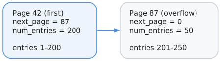
When a posting list exceeds one page, it chains to overflow pages:
Skip Pointers
Skip pointers enable O(log n) seeking within posting lists, dramatically speeding up multi-term AND queries.
Structure:
| Field | Size | Offset |
|---|---|---|
doc_id | 8 B | 0 |
byte_offset | 4 B | 8 |
entry_count | 4 B | 12 |
How they work:
Skip pointers are created every 128 entries (SKIP_INTERVAL). They record:
doc_id: The document ID at that entrybyte_offset: Where to jump in the posting dataentry_count: Number of entries before this pointer
Posting list with 500 entries:

Skip Pointers:
  [0] doc_id=1280, offset=512, count=128   ← entry 128
  [1] doc_id=2560, offset=1024, count=256  ← entry 256
  [2] doc_id=3840, offset=1536, count=384  ← entry 384

Seeking to doc_id 3000:
  1. Binary search skip pointers: find [1] (doc_id=2560 < 3000)
  2. Jump to offset 1024
  3. Linear scan from entry 256 to find doc_id 3000

Result: Skipped 256 entries instead of scanning all 300
Multi-term intersection optimization:
For AND queries like "database optimization":
- Sort terms by doc_freq (smallest first)
- Iterate through smallest posting list
- For each doc_id, use
skipTo()on other lists - Skip pointers let large lists jump ahead efficiently
Query: "the database" (AND)

"the":      10,000 documents
"database":    100 documents  ← Driver (smallest)

Without skip pointers: 10,000 + 100 = 10,100 iterations
With skip pointers:    100 + ~100 seeks = ~200 operations
4. Document Length Storage
BM25 scoring requires knowing each document's length. This is stored in a separate B+Tree:
| DocId | Length (tokens) |
|---|---|
| 1 | 150 |
| 2 | 45 |
| 3 | 892 |
| … | … |
Why store lengths?
BM25 penalizes long documents to prevent them from dominating results just because they contain more words. A 10,000-word document mentioning "database" once is less relevant than a 100-word document mentioning it once.
Statistics tracked:
total_docs: Total documents indexedtotal_tokens: Sum of all document lengthsavg_doc_length: Average tokens per document (for normalization)
5. BM25 Scoring
BM25 calculates a relevance score for each document.
The Formula
Score(D, Q) = Σ IDF(term) × TF_norm(term, D)
              for each term in query Q
Where:
IDF (Inverse Document Frequency):
IDF(term) = log((N - df + 0.5) / (df + 0.5) + 1)

N  = total number of documents
df = number of documents containing this term
Rare terms get higher IDF scores. If "quantum" appears in 5 of 10,000 documents, it's more significant than "the" appearing in 9,500.
TF_norm (Normalized Term Frequency):
TF_norm = (tf × (k1 + 1)) / (tf + k1 × (1 - b + b × (dl / avgdl)))

tf    = term frequency in this document
k1    = saturation parameter (default 1.2)
b     = length normalization (default 0.75)
dl    = document length
avgdl = average document length
Parameters
| Parameter | Default | Effect |
|---|---|---|
k1 | 1.2 | Controls term frequency saturation. Higher = more weight to repeated terms |
b | 0.75 | Length normalization. 0 = no normalization, 1 = full normalization |
Scoring Example
Corpus: 1000 documents, average length 200 tokens
Query: "database optimization"

Document 42:
  - Length: 150 tokens
  - "database" appears 3 times
  - "optimization" appears 1 time

Term: "database"
  - doc_freq = 50 (appears in 50 docs)
  - IDF = log((1000 - 50 + 0.5) / (50 + 0.5) + 1) = log(19.82) ≈ 2.99

  - tf = 3
  - dl/avgdl = 150/200 = 0.75
  - TF_norm = (3 × 2.2) / (3 + 1.2 × (1 - 0.75 + 0.75 × 0.75))
            = 6.6 / (3 + 1.2 × 0.8125)
            = 6.6 / 3.975
            ≈ 1.66

  - Score for "database" = 2.99 × 1.66 ≈ 4.96

Term: "optimization"
  - doc_freq = 10 (rarer term)
  - IDF = log((1000 - 10 + 0.5) / (10 + 0.5) + 1) ≈ 4.55

  - tf = 1
  - TF_norm = (1 × 2.2) / (1 + 1.2 × 0.8125) ≈ 1.12

  - Score for "optimization" = 4.55 × 1.12 ≈ 5.10

Total Score for Document 42 = 4.96 + 5.10 = 10.06
6. Search Flow
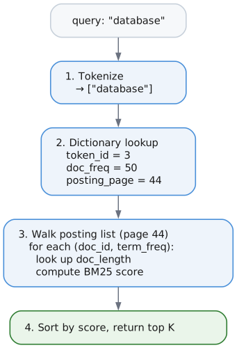
Single-Term Search
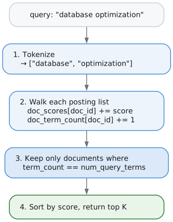
Multi-Term Search (AND Semantics)
OR Search
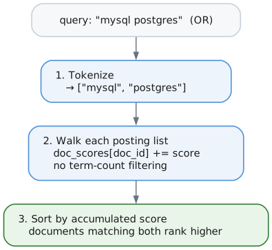
OR search returns documents matching any query term:
// Returns docs containing "mysql" OR "postgres" OR both
const results = try fts.searchOr("mysql postgres", 10);

// Or use explicit mode selection
const results = try fts.searchWithMode("mysql postgres", .@"or", 10);
NOT Search (Exclusions)
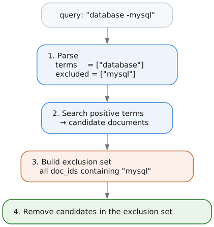
Prefix terms with - to exclude documents containing them:
// Find "database" docs that don't mention "mysql"
const results = try fts.searchWithMode("database -mysql", .@"and", 10);

// Multiple exclusions
const results = try fts.searchWithMode("database -mysql -oracle", .@"and", 10);
Phrase Search
Phrase search finds documents where terms appear adjacent and in order:
// Enable position storage in config
var fts = FtsIndex.init(allocator, &bp, &dict_tree, &lengths_tree, .{
    .store_positions = true,
});

// Search for exact phrase
const results = try fts.searchPhrase("quick brown fox", 10);
Query: "quick brown fox" (phrase)

Document 1: "The quick brown fox jumps"     ← MATCHES (adjacent: pos 1,2,3)
Document 2: "A quick red brown fox"         ← NO MATCH (not adjacent)
Document 3: "The brown quick fox"           ← NO MATCH (wrong order)
How it works:
-
Fetch the posting lists with positions:
Term Postings quickdoc 1 @ 1, doc 2 @ 1 browndoc 1 @ 2, doc 2 @ 3 foxdoc 1 @ 3, doc 2 @ 4 -
For each candidate document, check that the positions are adjacent:
Document Positions Adjacent? doc 1 quick@1,brown@2,fox@3Yes — 1+1=2 and 1+2=3, so it matches doc 2 quick@1,brown@3,fox@4No — 1+1=2 but brownis at 3
Note: Phrase queries require store_positions = true in FtsConfig. Without positions, searchPhrase() falls back to AND semantics.
Quoted Phrase Syntax
You can also use quoted strings in regular search() and searchWithMode() calls to automatically detect phrase queries:
// These are equivalent:
const results1 = try fts.searchPhrase("quick brown", 10);
const results2 = try fts.searchWithMode("\"quick brown\"", .@"and", 10);
Combining phrases with terms and exclusions:
// Phrase + additional term (AND mode)
// Matches documents with "quick brown" phrase AND term "jumps"
const results = try fts.searchWithMode("\"quick brown\" jumps", .@"and", 10);

// Phrase + exclusion
// Matches documents with "quick brown" phrase but NOT containing "fox"
const results = try fts.searchWithMode("\"quick brown\" -fox", .@"and", 10);

// Multiple phrases
// Matches documents with both phrases
const results = try fts.searchWithMode("\"quick brown\" \"lazy dog\"", .@"and", 10);

// Phrase with OR mode
// Matches documents with "quick brown" phrase OR term "rabbit"
const results = try fts.searchWithMode("\"quick brown\" rabbit", .@"or", 10);
Single-word quotes:
Single words in quotes are treated as regular terms (since a one-word phrase is just a term):
// These are equivalent:
const results1 = try fts.search("database", 10);
const results2 = try fts.searchWithMode("\"database\"", .@"and", 10);
Fuzzy Search
Fuzzy search finds documents even when query terms contain typos. It uses Levenshtein (edit) distance to match terms within a configurable threshold.
const fuzzy = @import("fts/fuzzy.zig");

// Search with typo tolerance (max 2 edits)
const results = try fts.searchFuzzy("databse", .{
    .max_distance = 2,      // Allow up to 2 edits
    .min_term_length = 4,   // Only fuzzy-match terms >= 4 chars
}, 10);
defer fts.freeResults(results);
// Matches documents containing "database" (edit distance 1)
How it works:
Query: "databse" (typo)
  ↓
Scan dictionary for terms within edit distance 2:
  - "database" (distance=1) ✓
  - "datastore" (distance=3) ✗
  ↓
Search matching terms with distance penalty:
  - Score("database") × penalty(1) = Score × 0.75
  ↓
Return ranked results
Distance penalty formula:
penalty = 1.0 - (distance / max_distance)²

Examples (max_distance = 2):
- distance 0: 1.00 (exact match)
- distance 1: 0.75 (25% penalty)
- distance 2: 0.00 (filtered out)
Levenshtein distance counts the minimum single-character edits needed:
- Insertion: "helo" → "hello" (distance 1)
- Deletion: "hello" → "helo" (distance 1)
- Substitution: "hello" → "hallo" (distance 1)
Note: Transpositions ("recieve" → "receive") count as 2 edits in standard Levenshtein.
Prefix/Wildcard Search
Prefix search finds documents containing terms that start with a given prefix. Use * as a suffix wildcard.
const prefix = @import("fts/prefix.zig");

// Search for terms starting with "optim" (matches "optimize", "optimization", "optimizer")
const results = try fts.searchWithPrefix("optim*", .{
    .min_prefix_length = 2,   // Minimum prefix length (prevents "a*" explosion)
    .max_expansions = 50,     // Maximum terms to expand
}, 10);
defer fts.freeResults(results);
How it works:
Query: "optim*"
  ↓
Calculate range bounds: ["optim", "optin")
  ↓
B+Tree range scan to find matching terms:
  - "optimization" ✓
  - "optimize" ✓
  - "optimizer" ✓
  ↓
Search all matching terms (like OR query)
  ↓
Return ranked results
Combining prefix with regular terms:
// AND semantics: documents must contain "systems" AND a term starting with "data"
const results = try fts.searchWithPrefix("systems data*", .{}, 10);
// Matches documents with both "systems" and "database"/"datastore"/"data"
Constraints:
- Suffix wildcards only (
optim*), not prefix wildcards (*tion) - No middle wildcards (
da*base) - Minimum prefix length configurable (default 2 chars)
- Maximum expansions capped to prevent explosion
Search Highlighting
Search highlighting returns text snippets with matched terms marked, enabling UI display of search results with context.
const highlight = @import("fts/highlight.zig");

const text = "The database stores data efficiently for optimal performance.";
const query_terms = [_][]const u8{ "database", "data" };

const result = try highlight.highlight(
    allocator,
    text,
    &query_terms,
    .{ .use_stemming = false },  // TokenizerConfig
    .{
        .context_chars = 80,      // Characters of context around matches
        .max_snippets = 3,        // Maximum snippets to return
        .merge_distance = 40,     // Merge snippets closer than this
        .prefix_marker = "<em>",  // Marker before matched terms
        .suffix_marker = "</em>", // Marker after matched terms
        .ellipsis = "...",        // Added when text is truncated
    },
);
defer highlight.freeResult(allocator, result);

// result.snippets[0].text = "The <em>database</em> stores <em>data</em> efficiently..."
// result.total_matches = 2
How it works:
Query terms: ["database", "data"]
Document: "The database stores data efficiently for optimal performance."
  ↓
Re-tokenize document with same config:
  - "database" at offset 4 → stems to "databas" or "database"
  - "data" at offset 20 → stems to "data"
  ↓
Match against query terms (stemmed comparison):
  - Match found at positions 4-12 and 20-24
  ↓
Group matches into snippets with context:
  - Single snippet with both matches (close together)
  ↓
Insert markers around matches:
  - "The <em>database</em> stores <em>data</em> efficiently..."
With stemming:
const text = "The runners were running fast in the marathon.";
const query_terms = [_][]const u8{"run"};  // Already stemmed query

const result = try highlight.highlight(
    allocator,
    text,
    &query_terms,
    .{ .use_stemming = true },  // Enable stemming
    .{ .prefix_marker = "**", .suffix_marker = "**" },
);
// "running" stems to "run" → match
// "runners" stems to "runner" → no match
// result.snippets[0].text = "The runners were **running** fast..."
Key design decisions:
- Re-tokenization approach: Document text is re-tokenized at query time (no storage overhead)
- Stemmed matching: Query terms are matched against stemmed document tokens
- Original text preserved: Markers wrap the original text, not stemmed forms
- Configurable markers: Default
<em>/</em>but customizable for any format - Snippet merging: Close matches combined into single snippets
Finding matches only (without snippets):
const matches = try highlight.findMatches(
    allocator,
    text,
    &query_terms,
    .{ .use_stemming = false },
);
defer highlight.freeMatches(allocator, matches);

for (matches) |match| {
    // match.start = byte offset of match start
    // match.end = byte offset of match end (exclusive)
    const matched_text = text[match.start..match.end];
}
7. Indexing Flow
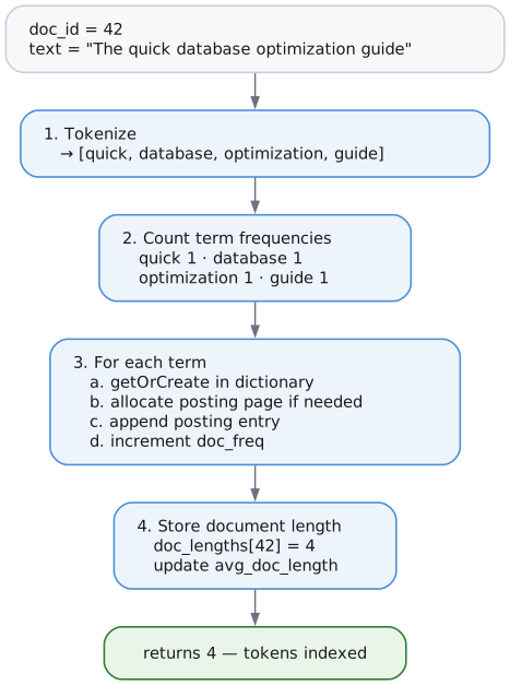
Nothing calls this directly any more. Writing an indexed property is what runs it, and section 15 covers how that happens. The mechanics below are unchanged: this is what one document costs whenever it is indexed.
Indexing one document
8. Data Structures Summary
In-Memory
| Structure | Purpose |
|---|---|
Tokenizer | Streaming text tokenization |
PostingIterator | Iterate posting list entries |
Bm25Scorer | Calculate relevance scores |
On-Disk (B+Trees)
| B+Tree | Key | Value |
|---|---|---|
| Dictionary | 4-byte scope prefix + token string | DictionaryEntry (24 bytes) |
| DocLengths | 4-byte scope prefix + DocId (8 bytes) | Length (4 bytes) |
| Reverse index | 4-byte scope prefix + DocId | Terms the document contributed |
| Index catalog | [kind, scope_id, property_id] | empty; the key is the record |
The scope prefix is what keeps one declared index out of another's way; section 14 explains it. The catalog shares its tree with the property indexes, under different kind discriminators.
On-Disk (Pages)
| Page Type | Content |
|---|---|
FTS_POSTING | Posting list entries (varint encoded) |
9. Limitations and Future Work
Current Limitations
- English-only stemming - Porter stemmer for English only (other languages skip stemming)
- One property per index - Searching several fields as one document means storing the combined text in a property and indexing that. The reasoning is in the design note: an index spanning
titleandbodywould maked.title @@ "x"match on body text, which is the confusion per-property indexes exist to remove. - Selectivity is per term, not per phrase - the estimate that chooses between two indexes is the rarest term's document frequency, which bounds an AND query correctly but says nothing about how often the terms occur together. Two predicates whose terms are individually common but jointly rare estimate as common.
- Fuzzy matching does not reach uncommitted text - Text written in the current transaction is matched by term presence rather than edit distance, because fuzzy expansion walks the committed dictionary.
Implemented Features
- Phrase queries -
searchPhrase("quick brown fox")with position verification - Boolean queries - AND (default), OR (
searchOr), NOT (-termsyntax) - Porter stemming -
use_stemming=truereduces words to roots (English) - Position indexing -
store_positions=truefor phrase queries - Skip pointers - O(log n) posting list intersection for multi-term queries
- Quoted phrase syntax - Parse
"exact phrase"in regular search() calls - Fuzzy search - Levenshtein distance for typo tolerance via
searchFuzzy() - Multi-language stop words - 11 languages supported (EN, DE, FR, ES, IT, PT, NL, SV, NO, DA, FI, RU)
- Prefix/wildcard search -
searchWithPrefix("optim*")expands to matching terms - Search highlighting -
highlight()returns snippets with matched terms marked - Document deletion -
removeDocument()with reverse index properly cleans posting lists and stats - Per-property indexes - one index per label and property, declared and then maintained by writes (sections 13 to 15)
- Relationship indexes - the same over a relationship type and property
- Index seek as the access path - a full-text predicate reads the index instead of filtering a label scan (section 16)
- Corpus statistics on disk - document count and average length survive a reopen, so scores do not depend on what the session happened to index
Planned Features
- Multi-language stemmers - Snowball stemmers for German, French, etc.
10. The Index Component Directly
This is the engine component, wired up by hand. It is here to show what the
pieces above do together, not as an API to use: nothing outside the storage layer
constructs an FtsIndex, and indexDocument is reached by writing an indexed
property rather than by calling it.
For the API you would actually use, see Full-Text Search (@@) and the full-text search guide.
const std = @import("std");
const lattice = @import("lattice");

pub fn main() !void {
    var gpa = std.heap.DebugAllocator(.{}){};
    const allocator = gpa.allocator();

    // Initialize storage (simplified)
    var bp = try BufferPool.init(allocator, &pm, 64 * 4096);
    var dict_tree = try BTree.init(allocator, &bp);
    var lengths_tree = try BTree.init(allocator, &bp);

    // Create FTS index with phrase query support
    var fts = FtsIndex.init(allocator, &bp, &dict_tree, &lengths_tree, .{
        .store_positions = true,  // Enable phrase queries
    });

    // Index documents
    _ = try fts.indexDocument(1, "Introduction to database systems");
    _ = try fts.indexDocument(2, "Advanced database optimization techniques");
    _ = try fts.indexDocument(3, "Web development with JavaScript");
    _ = try fts.indexDocument(4, "Database performance and MySQL tuning");

    // Basic AND search (all terms must match)
    const results1 = try fts.search("database optimization", 10);
    defer fts.freeResults(results1);
    // Returns doc 2 (contains both terms)

    // OR search (any term matches)
    const results2 = try fts.searchOr("mysql postgres", 10);
    defer fts.freeResults(results2);
    // Returns doc 4 (contains "mysql")

    // NOT search (exclusions with -prefix)
    const results3 = try fts.searchWithMode("database -mysql", .@"and", 10);
    defer fts.freeResults(results3);
    // Returns docs 1, 2 (contain "database" but not "mysql")

    // Phrase search (exact sequence)
    const results4 = try fts.searchPhrase("database systems", 10);
    defer fts.freeResults(results4);
    // Returns doc 1 (has "database systems" as adjacent phrase)

    // Quoted phrase syntax (alternative to searchPhrase)
    // Phrase "database optimization" + term "advanced"
    const results5 = try fts.searchWithMode("\"database optimization\" advanced", .@"and", 10);
    defer fts.freeResults(results5);
    // Returns doc 2 (has phrase "database optimization" AND term "advanced")

    // Fuzzy search (typo tolerance)
    const results6 = try fts.searchFuzzy("databse", .{
        .max_distance = 2,
        .min_term_length = 4,
    }, 10);
    defer fts.freeResults(results6);
    // Returns docs with "database" (edit distance 1 from "databse")

    for (results1) |result| {
        std.debug.print("Doc {}: score {d:.2}\n", .{ result.doc_id, result.score });
    }
}
11. Serialization Pattern
All on-disk structures use extern struct with compile-time size assertions:
/// Good: Self-documenting, compile-time verified
pub const PostingPageHeader = extern struct {
    token_id: TokenId,
    num_entries: u32,
    next_page: PageId,
    num_skip_pointers: u16,
    flags: u16,
    data_start: u32,

    comptime {
        std.debug.assert(@sizeOf(PostingPageHeader) == 20);
    }

    pub fn read(data: []const u8) PostingPageHeader {
        return std.mem.bytesAsValue(PostingPageHeader, data[OFFSET..][0..@sizeOf(PostingPageHeader)]).*;
    }

    pub fn write(self: *const PostingPageHeader, data: []u8) void {
        @memcpy(data[OFFSET..][0..@sizeOf(PostingPageHeader)], std.mem.asBytes(self));
    }
};
Why this pattern?
- No magic numbers - Field layout is defined by the struct, not manual offsets
- Compile-time verification -
comptimeblock catches size mismatches immediately - Self-documenting - Struct fields serve as documentation
- Consistent with codebase - WAL, PageHeader, FileHeader all use this pattern
Alignment considerations:
When structs contain u64 fields, use explicit padding and order fields largest-first:
pub const DictionaryEntry = extern struct {
    total_freq: u64,   // 8 bytes - largest first (requires 8-byte alignment)
    token_id: u32,     // 4 bytes
    doc_freq: u32,     // 4 bytes
    posting_page: u32, // 4 bytes
    _padding: u32 = 0, // 4 bytes - explicit trailing padding

    comptime {
        std.debug.assert(@sizeOf(DictionaryEntry) == 24);
    }
};
13. Declared Indexes
An index covers one label and one property. Nothing is indexed until you say so.
try db.createNodeFtsIndex("Document", "body");
Declaring reads body from every node already carrying Document and indexes
it, so adding an index to a database full of documents makes them searchable
immediately rather than only affecting what arrives afterwards. That mirrors what
createNodePropertyIndex does, for the same reason: an index that only covers
future writes is a trap.
Where a declaration lives
Declarations go in the same B+Tree as the property index catalog, under their own kind discriminators:
| Kind | Meaning |
|---|---|
| 1 | node property index |
| 2 | edge property index |
| 3 | node full-text index |
| 4 | edge full-text index |
The key is [kind (1 byte), scope_id (2 bytes big-endian), property_id (2 bytes big-endian)] and the value is empty — the key is the whole record. scope_id is
a label for a node index and a relationship type for an edge one; both are symbol
ids from the same table the rest of the engine uses.
Sharing the catalog tree was free. The key already began with a kind byte, so
adding two more kinds needed no format change and no new tree. Big-endian is what
makes a range scan over one kind possible: [3] to [4] covers every node
full-text declaration and nothing else.
Why not multiple properties per index
Storing several properties as one document is easy. Asking for it is not. If an
index merged title and body, then WHERE d.title @@ "x" would match documents
whose body contained the term, and the property name would be lying — which is
the exact confusion per-property indexes exist to remove. Reusing property access
as the query syntax requires one property per index.
Somebody who wants several fields ranked as one document stores the combined text in a property and indexes that. The text is then visible in the database, where it can be read and rebuilt, instead of living only inside an index.
14. One Set of Trees, Many Indexes
Every declared index shares the dictionary, document-length, and reverse-index
trees. Without something separating them, a term indexed for title would be
found by a search of body.
Every key written for an index carries a four-byte prefix naming it:
[kind (1), scope_id (2 BE), property_id (1)] ++ the key the store wanted
So bread in Document.title and bread in Document.body are two different
keys in one tree, and a range over a prefix walks one index's terms and stops.
Why a view rather than a prefix argument
The prefix is applied by a wrapper — ScopedTree — that the stores hold in place
of a raw B+Tree. The stores' key-building code did not change at all.
The alternative was passing a prefix into each place that builds a key, of which there are about a dozen across three files. Missing one would not fail to compile. It would write an entry the matching read could never find, or read another index's entries. One place to get right beats twelve places to remember.
The prefix arithmetic
Walking one index means ranging from its prefix to the next one. Computing "the
next prefix" has a trap: a prefix ending in 0xFF has to carry into the byte
before it. Incrementing the last byte alone wraps to zero, producing an upper
bound below the lower one, and the index reads as empty. That carry is a
function with its cases tested rather than arithmetic written inline twice.
Where the prefix comes off again
Reads strip the prefix before returning keys, because callers want the term. This matters more than it sounds: fuzzy search measures edit distance against the term text, so four bytes of index identity on the front puts every term far outside any sensible distance and nothing ever matches. The stripping lives in the iterator, next to the prefixing, so the two cannot drift apart.
15. Keeping Indexes Current
Writing an indexed property maintains the index. There is no separate indexing call, and nothing to forget.
Create, update, and delete all funnel through one function per entity kind, where an empty old state means a create and an empty new state means a delete. Eight call sites reach those two functions, which is eight fewer places that could each decide what a change means.
What is indexed
Only string properties. A number, a list, or an absent property contributes
nothing. Rendering 42 as "42" so a text search could match it would be a
different feature with different rules, and doing half of it silently would make
results hard to explain.
Unchanged text is left alone
An update whose indexed text did not change skips the index entirely. Without that, writing any property on an entity would reindex its longest indexed string, and the cost of an unrelated write would scale with how much text the entity happens to carry.
Recovery
Redo replays into the stores directly rather than through the write path, so nothing maintains the indexes while it runs — the same situation the property indexes are already in. After a redo, each declared index is cleared and rebuilt.
The clear works by scope prefix rather than by walking documents. An entity the redo deleted is no longer there to walk, so walking would leave its terms behind to keep matching. Deleting by prefix is a batched collect-then-delete, because the tree's iterator pins a leaf and holds a slot in it, which makes deleting during iteration unsafe; a fixed batch keeps memory flat rather than proportional to what is often the largest structure in the database.
Posting pages of a cleared index stay allocated. Nothing points at them once the dictionary entries naming them are gone, so it is wasted space rather than wrong data, and reclaiming it needs page reuse the store does not have yet.
16. Search as an Access Path
A @@ predicate is planned as the way into the data, not as a filter over a scan.
Why per-property indexing is what makes this possible
A Document.body index contains only Document nodes. The index is already
label-scoped, so reading it does the label scan's job and answers the text
question at the same time. The older design — one index spanning every node —
could not have done this: it had no idea which nodes carried which label, so it
could only ever filter a scan somebody else produced.
The measurement
Eight thousand documents, a query matching one of them:
| time | |
|---|---|
| the index lookup alone | 31 µs |
| scanning the label and keeping what the index named | 72 ms |
the same predicate under an AND, filtered per row | 216 ms |
The scan cost the whole corpus to answer a question the index had already answered. Seeking instead:
| before | after | |
|---|---|---|
@@ 'rare' | 72 ms | 105 µs |
@@ 'rare' AND … | 216 ms | 105 µs |
@@ 'common' AND … | 21.3 s | 320 ms |
Selective queries also stopped growing with the corpus — 65 µs, 80 µs, 105 µs from five hundred to eight thousand documents, against 3.9 ms, 17 ms, 72 ms before.
When it applies
Only in conjunctive positions: the whole WHERE, or a branch of an AND.
Under an OR the planner deliberately does not seek. The other branch can admit
entities the index never names, so seeking would silently drop rows. There is a
test asserting that an OR plans a label scan, because the reason is not visible
from reading the planner and the shape looks like a missed optimisation.
The predicate also has to name the entity the pattern is about. Where the variable is already bound by an upstream expand, the input decides which rows exist and the index can only filter them.
The filter that remains
What cannot be sought is still answered by evaluating @@ per row. That path
consults the index once per query rather than once per row, keyed on the
resolved index and the query text, and held for one execution.
Without it the filter was quadratic in the corpus: its cost against a scan grew 8.4x, 22.2x, then 152.1x as the corpus grew, and is now a flat 2.4x, 2.7x, 2.3x.
Reusing a search within one execution is the same assumption the scanning operators have always made — they search once when they open and use that result for every row they emit. The cache matches that granularity rather than inventing a stricter or a looser rule.
Choosing between two ways in
d.title @@ "the" AND d.body @@ "sourdough" offers two ways into the data, and
they are not equally cheap. Starting from a word most documents share means
reading the corpus to discard it; starting from a rare one means reading almost
nothing.
The dictionary already records, for every term, how many documents contain it. An AND query cannot match more documents than its rarest term appears in, so the minimum of those counts is a real upper bound rather than a guess — and a term absent from the dictionary gives zero, which is exact. Each candidate costs one B-tree lookup per term to estimate.
The choice is made when the query runs, not when it is planned, for two reasons. A query whose text arrives as a parameter has nothing to estimate at plan time. And a cached plan would carry a decision made against whatever the data looked like when it was first planned.
Choosing at execution is safe because the filter above the seek applies the whole condition regardless of which candidate was read, so the choice can only affect how much work is done, never which rows come back.
Candidates are confined to one label. The label the access path guarantees is the one whose filter the planner skips, and which candidate runs is not known until it runs; candidates spanning two labels would mean skipping a filter the chosen path does not satisfy. That was a real defect during development — a pattern asking for two labels returned entities carrying only one — and it survived two tests that passed for an unrelated reason before a negative control exposed it.
Measured on eight thousand documents, one matching row:
| query | before | after |
|---|---|---|
| rare predicate written first | 4.3 ms | 4.3 ms |
| common predicate written first | 244 ms | 4.2 ms |
The point is not only the 59x. It is that the two rows now agree: how the author ordered the predicates no longer decides what the query costs.
Disjunctions
Several @@ predicates on one variable joined by OR are planned as a single
operator that reads each index once and unions the results. A document found by
more than one takes its best score rather than a sum: two properties matching is
not evidence that either matched twice as well, and adding them would rank a
document matching both weakly above one matching a single property strongly.
Mixing kinds is refused. d.title @@ "x" OR r.note @@ "x" cannot be one union,
because one operator filters one slot and a slot holds a node or an edge. That
query still answers correctly, through the row filter.
12. File Reference
| File | Purpose |
|---|---|
src/fts/tokenizer.zig | Text tokenization, normalization, language config |
src/fts/stopwords.zig | Multi-language stop word lists (11 languages) |
src/fts/dictionary.zig | Token → TokenId mapping via B+Tree, range iteration |
src/fts/posting.zig | Posting list storage with varint encoding, entry removal |
src/fts/scorer.zig | BM25 scoring, document length storage |
src/fts/index.zig | Main FtsIndex coordinator, boolean/phrase/fuzzy/prefix search |
src/fts/stemmer.zig | Porter stemmer algorithm (English), language routing |
src/fts/fuzzy.zig | Levenshtein distance, fuzzy term expansion |
src/fts/prefix.zig | Prefix/wildcard search, upper bound calculation |
src/fts/highlight.zig | Search result highlighting, snippet extraction |
src/fts/reverse_index.zig | doc_id → terms mapping for document deletion |
src/fts/catalog.zig | Declared indexes: kind, scope, property |
src/fts/scoped_tree.zig | Prefixing view that keeps declared indexes apart |
src/query/operators/fts.zig | Index seek and filtering operators |