LatticeDB
Embedded property graph with native vector, full-text, and durable event primitives.
LatticeDB is a single-file local database for connected, semantic, and textual data. It lets applications traverse relationships, run HNSW vector similarity, run BM25 full-text search, and consume durable graph/application events from the same file.
- One file. Your entire database is a single portable file. No server, no configuration.
- One query layer. Graph traversal, HNSW vector similarity, and BM25 full-text — in one query.
- One event log. Durable named streams and the built-in graph changefeed share the same transaction/WAL path as graph writes.
- Sub-millisecond. 0.13 us node lookups. 0.83 ms vector search at 1M vectors with 100% recall.
-- Find chunks similar to a query, traverse to their document, then to the author
MATCH (chunk:Chunk)-[:PART_OF]->(doc:Document)-[:AUTHORED_BY]->(author:Person)
WHERE chunk.embedding <=> $query_vector < 0.3
  AND doc.content @@ "neural networks"
RETURN doc.title, chunk.text, author.name
ORDER BY chunk.embedding <=> $query_vector
LIMIT 10
Features
Graph
- Nodes and edges with labels and arbitrary properties
- Multi-hop traversal, variable-length paths (
*1..3) - ACID transactions with snapshot isolation
- MERGE, WITH, UNWIND, aggregations (
count,sum,avg,min,max,collect)
Vector Search
- HNSW approximate nearest neighbor with configurable M, ef
- Built-in hash embeddings or HTTP client for Ollama/OpenAI
- Batch insert for bulk loading
Full-Text Search
- BM25-ranked inverted index with tokenization and stemming
- Fuzzy search with configurable Levenshtein distance
Cypher Query Language
- MATCH, WHERE, RETURN, CREATE, DELETE, SET, REMOVE
- ORDER BY, LIMIT, SKIP, DETACH DELETE
- Vector distance operator:
<=> - Full-text search operator:
@@ - Parameters:
$name
Operations
- Single-file storage with write-ahead log for crash recovery
- Durable streams and semantic graph changefeeds
- Zero configuration — open a file and start working
- Clean C API; Python, TypeScript, and Go bindings wrap it
Use Cases
- RAG Systems — Vector search finds relevant chunks, graph traversal gathers context
- Knowledge Graphs — Linked notes and documents with semantic search
- AI Agents — Persistent memory with relationship awareness
- Local Development — Lightweight alternative to Neo4j or Weaviate for prototyping
Getting Started
Head to the Installation page to install LatticeDB, then follow the Quick Start guide to build your first knowledge graph.
Installation
CLI
curl -fsSL https://raw.githubusercontent.com/jeffhajewski/latticedb/main/dist/install.sh | bash
Python
pip install latticedb
Requires Python 3.9+ and NumPy. The native shared library (liblattice.dylib / liblattice.so) must be available on the system.
TypeScript / Node.js
npm install @hajewski/latticedb
Requires Node.js 18+. The native shared library must be available on the system.
Building from Source
LatticeDB is written in Zig with zero dependencies.
git clone https://github.com/jeffhajewski/latticedb.git
cd latticedb
zig build                  # build everything
zig build test             # run tests
zig build -Doptimize=ReleaseFast   # optimized build
Build the shared library for language bindings:
zig build shared
This produces liblattice.dylib (macOS) or liblattice.so (Linux).
See Building from Source for more details.
Quick Start
This guide walks through creating a small knowledge graph with documents and authors, storing embeddings, indexing text, and querying across all three search modes.
The fastest thing that works
Before the full example, here is the smallest one. Pass :memory: as the path and
you get a real database with nothing to create and nothing to clean up:
from latticedb import Database

db = Database(":memory:")
db.query("CREATE (a:Person {name: 'Alice'})")
print(db.query("MATCH (p:Person) RETURN p.name"))
Everything works the same as a database on disk — transactions, indexes, vector and text search — it just disappears when you close it. It is the easiest way to try a query, and it is what tests usually want. See In-Memory Databases.
Swap ":memory:" for a filename when you want to keep the results.
Python
from latticedb import Database, hash_embed

with Database("knowledge.db", create=True, enable_vector=True, vector_dimensions=128) as db:

    # --- Build the graph ---
    db.create_node_fts_index("Chunk", "text")

with db.write() as txn:
        # Create authors
        alice = txn.create_node(labels=["Person"], properties={"name": "Alice", "field": "ML"})
        bob = txn.create_node(labels=["Person"], properties={"name": "Bob", "field": "Systems"})
        txn.create_edge(alice.id, bob.id, "COLLABORATES_WITH")

        # Create documents with chunks
        for title, text, author in [
            ("Attention Is All You Need", "The transformer architecture uses self-attention...", alice),
            ("Scaling Laws for LLMs", "We find that model performance scales predictably...", alice),
            ("Log-Structured Merge Trees", "LSM trees optimize write-heavy workloads...", bob),
        ]:
            doc = txn.create_node(labels=["Document"], properties={"title": title})
            chunk = txn.create_node(labels=["Chunk"], properties={"text": text})

            # The chunk's text is indexed because Chunk.text is declared below.
            txn.set_vector(chunk.id, "embedding", hash_embed(text, dimensions=128))

            txn.create_edge(chunk.id, doc.id, "PART_OF")
            txn.create_edge(doc.id, author.id, "AUTHORED_BY")

        txn.commit()

    # --- Query: vector search + text match + graph traversal ---
    results = db.query("""
        MATCH (chunk:Chunk)-[:PART_OF]->(doc:Document)-[:AUTHORED_BY]->(author:Person)
        WHERE chunk.embedding <=> $query < 0.5
        RETURN doc.title, chunk.text, author.name
        ORDER BY chunk.embedding <=> $query
        LIMIT 5
    """, parameters={"query": hash_embed("transformer attention mechanism", dimensions=128)})

    for row in results:
        print(f"{row['doc.title']} by {row['author.name']}")

    # --- Full-text search ---
    for r in db.fts_search("Chunk", "text", "self-attention transformer"):
        print(f"Node {r.node_id}: score={r.score:.4f}")

    # --- Aggregations ---
    stats = db.query("""
        MATCH (doc:Document)-[:AUTHORED_BY]->(p:Person)
        RETURN p.name, count(doc) AS papers
        ORDER BY papers DESC
    """)
    for row in stats:
        print(f"{row['p.name']}: {row['papers']} papers")
TypeScript
import { Database, hashEmbed } from "@hajewski/latticedb";

const db = new Database("knowledge.db", {
  create: true,
  enableVector: true,
  vectorDimensions: 128,
});
await db.open();

// Build a graph
await db.write(async (txn) => {
  const alice = await txn.createNode({
    labels: ["Person"],
    properties: { name: "Alice", field: "ML" },
  });
  const doc = await txn.createNode({
    labels: ["Document"],
    properties: { title: "Attention Is All You Need" },
  });
  const chunk = await txn.createNode({
    labels: ["Chunk"],
    properties: { text: "The transformer architecture uses self-attention..." },
  });

  await txn.setVector(chunk.id, "embedding", hashEmbed("transformer self-attention", 128));

  await txn.createEdge(chunk.id, doc.id, "PART_OF");
  await txn.createEdge(doc.id, alice.id, "AUTHORED_BY");
});

// Query across vector search + graph traversal
const results = await db.query(
  `MATCH (chunk:Chunk)-[:PART_OF]->(doc:Document)-[:AUTHORED_BY]->(author:Person)
   WHERE chunk.embedding <=> $query < 0.5
   RETURN doc.title, chunk.text, author.name
   ORDER BY chunk.embedding <=> $query
   LIMIT 5`,
  { query: hashEmbed("attention mechanism", 128) }
);

for (const row of results.rows) {
  console.log(`${row["doc.title"]} by ${row["author.name"]}`);
}

await db.close();
Next Steps
- Core Concepts — understand the data model
- Cypher Overview — learn the query language
- Data Export — export to JSON, JSONL, CSV, or DOT
- Building a RAG System — end-to-end tutorial
The lattice Command
Installing LatticeDB gives you a lattice command. It is the fastest way to create a
database, poke around in one, and move data in and out — no code required.
Every command follows the same shape:
lattice <command> [options] <path>
The path is the database file. Almost every command needs one; version, help, and
update are the exceptions.
If you ever forget what something does, ask it:
lattice help            # everything at a glance
lattice export --help   # detail for one command
A quick tour
Here is the whole thing in five commands. Create a database, put something in it, and look at what you have.
lattice create social.lattice
lattice exec social.lattice --query="CREATE (a:Person {name: 'Alice', age: 30})"
lattice exec social.lattice --query="CREATE (b:Person {name: 'Bob', age: 41})"
lattice exec social.lattice --query="MATCH (a:Person {name:'Alice'}), (b:Person {name:'Bob'}) CREATE (a)-[:KNOWS {since: 2020}]->(b)"
lattice count social.lattice
That last command prints:
┌───────────┬────────────┐
│ Type      │ Count      │
├───────────┼────────────┤
│ Nodes     │          2 │
│ Edges     │          1 │
│ Labels    │          1 │
│ EdgeTypes │          1 │
└───────────┴────────────┘
Creating a database
create makes a new database file. On its own it gives you a graph with full-text
search turned on:
lattice create social.lattice
Created database: social.lattice
  Full-text search enabled
If you plan to store embeddings, turn the vector index on at creation time and say how many dimensions your vectors have. This has to be decided up front, because the index is built into the file:
lattice create embeddings.lattice --enable-vector --vector-dims=1536
| Option | What it does |
|---|---|
--enable-vector | Turn on the vector index for similarity search |
--vector-dims=<n> | How many numbers are in each vector, 1 to 4096 (default 128) |
--enable-fts | Turn on full-text search — already the default |
--no-fts | Leave full-text search out |
--cache-size=<mb> | How much memory to keep pages in, in MB (default 64) |
--page-size=<bytes> | Page size, 4096 to 65535 (default 4096) |
Pick --vector-dims to match whatever produces your embeddings. OpenAI's
text-embedding-3-small gives you 1536 numbers per vector, so that is the number you
would use.
Running queries
There are two ways to run Cypher. Use exec for one query, and query when you want
to sit and explore.
One query at a time
lattice exec social.lattice --query="MATCH (p:Person) RETURN p.name, p.age"
You can keep a longer query in a file instead of fighting with shell quoting:
lattice exec social.lattice --file=report.cypher
An interactive shell
lattice query social.lattice
This drops you into a prompt where you can type queries and see results immediately. It also understands a few commands of its own, all starting with a dot:
| Command | What it does |
|---|---|
.help | List these commands |
.labels | List every node label |
.types | List every edge type |
.schema | Show what the data looks like |
.format table|json|csv | Change how results are printed |
.timing on|off | Show how long each query took |
.exit or .quit | Leave |
Looking at what is in there
Four commands answer "what is actually in this database?".
count gives you the totals, as shown in the tour above.
labels and types list the node labels and edge types, with how many of each:
lattice labels social.lattice
┌────────┬────────────┐
│ Label  │ Count      │
├────────┼────────────┤
│ Person │          2 │
└────────┴────────────┘
1 label(s)
schema puts both together. LatticeDB does not make you declare a schema up front, so
this is worked out by looking at the data that is actually there:
lattice schema social.lattice
Schema
══════

Node Labels:
  (:Person) - 2 node(s)

Edge Types:
  [:KNOWS] - 1 edge(s)

Total: 1 label(s), 1 edge type(s)
info describes the file rather than its contents — size, counts, and which features
it was built with:
lattice info social.lattice
Database: social.lattice
─────────────────────────────
Size:         68 KB
Nodes:        2
Edges:        1
Format:       v3
FTS:          enabled
Moving data in and out
Importing
import reads JSON or CSV:
lattice import social.lattice --file=people.json
Importing people.json into social.lattice...
Import complete
  Nodes imported: 2
  Edges imported: 1
JSON should have a nodes array and an edges array:
{
  "nodes": [
    {"id": "n1", "labels": ["Person"], "properties": {"name": "Carol", "age": 29}},
    {"id": "n2", "labels": ["Person"], "properties": {"name": "Dan", "age": 35}}
  ],
  "edges": [
    {"source": "n1", "target": "n2", "type": "KNOWS", "properties": {"since": 2021}}
  ]
}
CSV needs two files, one for nodes and one for edges. Columns starting with an underscore have special meaning; everything else becomes a property:
_id,_labels,name,age
n1,"Person;Employee",Alice,30
_source,_target,_type,since
n1,n2,KNOWS,2020
Two options are worth knowing about for large imports:
| Option | What it does |
|---|---|
--batch-size=<n> | Commit every N items instead of all at once (default 1000) |
--on-error=skip | Skip records that fail instead of giving up on the whole import |
--on-error=skip applies records one at a time, so the good rows still land. That is
slower, but it means one bad row in a large file does not cost you the import.
Exporting
export writes JSON, JSONL, CSV, or DOT. It picks the format from the file extension:
lattice export social.lattice --file=backup.json
lattice export social.lattice --file=graph.jsonl
lattice export social.lattice --file=people.csv --labels=Person
lattice export social.lattice --file=graph.dot
DOT is the format Graphviz reads, so you can turn a small graph into a picture:
digraph G {
  n1 [label="1 : Person"];
  n2 [label="2 : Person"];
  n1 -> n2 [label="KNOWS"];
}
You can narrow what gets exported with --labels=Person,Company, or export the result
of a query instead of the whole graph with --query="...".
Dumping
dump writes the whole database to standard output as JSON, in a stable order:
lattice dump social.lattice > snapshot.json
Because the ordering is fixed, two dumps of the same data produce identical files. That
makes dump useful in tests and for spotting what changed between two databases with a
plain diff.
Looking after a database
Checking for damage
check opens the file read-only and verifies the checksum stored on every page:
lattice check social.lattice
Database file checks passed
  Pages checked: 16
  Note: sibling WAL file exists but was not validated
One thing to be aware of: this checks the main database file only. If a write-ahead log
file is sitting next to it, check will tell you it exists but will not look inside it.
The write-ahead log is the file LatticeDB appends changes to before applying them, so
that a crash cannot leave the database half-written.
Backing up
backup copies a database to another file without closing it:
lattice backup social.lattice --file=/backups/social-2026-08-25.lattice
Backed up social.lattice to /backups/social-2026-08-25.lattice
  Bytes copied:    65536
  Pages:           16
  Pages flushed:   0
  Duration:        1 ms
Pending writes are folded into the file before the copy starts, so what you get is a complete database on its own — you can open it directly, and it needs no write-ahead log beside it.
The copy is written next to the destination and renamed into place only once it is finished. An interrupted backup leaves nothing that looks usable, rather than a truncated file you discover is bad when you need it.
Two things to know. The backup captures the database as of the moment it starts, so writes that land during it are not included. And it will refuse to run while a transaction is open, because a copy taken while writes land underneath it is torn in ways no later check would catch.
Do not back up by copying the file yourself while the database is open. The
write-ahead log holds committed data that is not in the main file yet, so
copying just the main file gives you a database that opens and then fails on
query, and copying both files catches them at different instants and fails on
open. Neither announces itself at copy time — you find out at restore. Use
backup, or stop the process first.
Shipping changes somewhere else
A backup taken by hand is only as good as the last time you remembered to take
one. replicate keeps a directory up to date with a database, so a failed disk
costs you the last few seconds of writes rather than everything since your last
copy:
lattice replicate social.lattice --to=/mnt/backup/social
Started generation 1 for social.lattice in /mnt/backup/social
  Snapshot bytes:  73728
  Generation:      1
  Frames shipped:  0
  Bytes shipped:   0
  Duration:        2 ms
The first pass copies the whole database. Every pass after that copies only the changes since the last one, which is why running it often is cheap:
Shipped social.lattice to /mnt/backup/social
  Generation:      1
  Frames shipped:  5
  Bytes shipped:   20480
  Duration:        2 ms
A pass with nothing to ship is normal and is not an error. It tells you so and exits successfully, which means you can put this on a timer without your logs filling up with things that look like failures.
Add --follow to leave it running instead:
lattice replicate social.lattice --to=/mnt/backup/social --follow --interval=30
Inside the destination you will find a manifest, a snapshot, and the changes that have arrived since:
/mnt/backup/social/manifest.json
/mnt/backup/social/gen-0000000001/snapshot.lattice
/mnt/backup/social/gen-0000000001/frames/0000000012-0000000016.frames
Every so often LatticeDB folds pending changes into the database file and starts the log over. When that happens, replication starts a generation: a fresh snapshot, followed by the changes that came after it. Older generations are left alone, because restoring to a moment inside one still needs them.
There is one important limit. This command opens the database, and LatticeDB does
not lock a database across processes, so you must not point it at a database
another process has open. If you want to replicate a database while your
application is using it, call replicateTo on the handle your application
already has, and use this command for the case where nothing else is running.
Getting a database back
restore turns a replication directory back into a database:
lattice restore /mnt/backup/social --output=recovered.lattice
Restored /mnt/backup/social to recovered.lattice
  Generation:      1
  Segments:        2
  Frames replayed: 20
  Bytes written:   73728
  Restored to:     2026-08-25T22:44:18Z
  Duration:        468 ms
It copies the snapshot, replays the changes shipped after it, and folds the result into one file. You can open that file, copy it, or move it, with nothing else beside it that has to be kept together with it.
To go back to an earlier moment, say when:
lattice restore /mnt/backup/social --output=recovered.lattice --at="2026-08-25T14:00:00Z"
Times are read as UTC, so a restore means the same thing wherever you run it. A bare date works too and means midnight.
There is a limit worth understanding here. What you get is the state as of the last replication pass at or before the moment you asked for, not the state at that exact instant. If you replicate every thirty seconds, you can rewind to within thirty seconds. That is why the output tells you the moment it actually restored to, rather than repeating the one you asked for.
restore will not write over a file that already exists unless you pass
--force, because the thing most likely to be sitting at the output path is a
database somebody still wants.
Flushing pending writes
Changes are written to a write-ahead log first, and folded into the database file
later. checkpoint does that folding on demand and then resets the log:
lattice checkpoint social.lattice
Checkpointed database: social.lattice
  Pages flushed:   0
  Checkpoint LSN:  2
  WAL truncated:   yes
  Duration:        0 ms
You mostly do not need this. A database checkpoints itself as the log grows, and again when it closes. It is worth running by hand in two situations: before copying a database file, so the copy is complete on its own, and on a database that has been open a very long time under heavy writes, if you want to pick the moment the flush happens rather than let it land mid-request.
This is not the same as compact. Checkpointing shrinks the log, not the
database file.
Reclaiming space
Deleting a lot of data leaves free pages behind, and the file stays the same size
because those pages are kept for reuse. compact hands the unused ones at the end of
the file back to the operating system:
lattice compact social.lattice
Compacted database: social.lattice
  Pages before:    17
  Pages after:     17
  Pages removed:   0
  Bytes reclaimed: 0
Nothing was reclaimed here because nothing had been deleted. A few things are worth knowing before you run it on real data:
- It only truncates free pages at the end of the file. Free pages in the middle stay where they are and get reused normally, so a file with holes in the middle will not shrink much.
- Live pages are never moved, which is what makes it safe to interrupt.
- It will refuse to run on a read-only database, or while any transaction is open.
Updating
update replaces your installed copy with the latest release:
lattice update
Working without a file
Pass :memory: instead of a path and the database lives only in memory:
lattice exec :memory: --query="CREATE (n:Note {t: 'scratch'}) RETURN n"
Nothing is written to disk and nothing survives the command, which makes it handy
for trying a query out or checking what some Cypher does. There is no file to
lock, so --no-lock means nothing here.
One process at a time
A database can only be open in one process at a time. If you run a command against a database your application already has open, it stops before touching anything:
Error: social.lattice is open in another process. Close it first, or pass
--no-lock if you are certain nothing is writing to it.
A command that writes needs the database to itself, and a command that only reads is also refused while something else is writing. That second part surprises people, so it is worth saying why: a reader in another process cannot see the writer's pending changes, and would be reading a file that is being rewritten underneath it. The answer it gave you would be stale at best.
Any number of read-only commands can run at once against a database nobody is writing.
Every command accepts --no-lock, which skips the check. It exists for
filesystems where locking does not work, such as some network filesystems. It
does not make concurrent access safe — it removes the thing that was going to
tell you it was not.
Output formats
Most commands can print in a different format, which is what you want when something else is going to read the output:
lattice count social.lattice --format=json
lattice count social.lattice --format=csv
type,count
nodes,2
edges,1
labels,1
edge_types,1
table is the default and is meant for reading. json and csv are meant for piping
somewhere else:
lattice exec social.lattice --query="MATCH (p:Person) RETURN p.name" --format=json | jq
Every command at a glance
| Command | What it does |
|---|---|
create <path> | Make a new database |
info <path> | Show file size, counts, and enabled features |
compact <path> | Give free pages at the end of the file back to the OS |
checkpoint <path> | Flush pending writes into the file and reset the log |
backup <path> | Copy to another file while the database stays open |
replicate <path> | Keep a directory up to date with the database |
restore <dir> | Rebuild a database from a replication directory |
check <path> | Verify page checksums in the main file |
query <path> | Open an interactive Cypher shell |
exec <path> | Run one query and exit |
import <path> | Load data from JSON or CSV |
export <path> | Write data to JSON, JSONL, CSV, or DOT |
dump <path> | Print the whole database as canonical JSON |
labels <path> | List node labels and their counts |
types <path> | List edge types and their counts |
schema <path> | Show the shape of the data |
count <path> | Show node and edge totals |
update | Update your LatticeDB installation |
version | Print the version and file format version |
help | Show usage |
Where to go next
- Quick Start for the same ideas from Python or TypeScript
- Core Concepts for what nodes, edges, and properties actually are
- Cypher Overview for the query language itself
Core Concepts
Property Graph
LatticeDB stores data as a property graph: a collection of nodes connected by edges, where both nodes and edges can have labels and key-value properties.
Nodes
A node represents an entity. Each node has:
- A unique ID (assigned automatically)
- One or more labels that categorize it (e.g.,
Person,Document,Chunk) - Zero or more properties — key-value pairs (e.g.,
name: "Alice",age: 30)
alice = txn.create_node(
    labels=["Person"],
    properties={"name": "Alice", "age": 30}
)
Edges
An edge represents a relationship between two nodes. Each edge has:
- A source node and a target node
- An edge type (e.g.,
KNOWS,AUTHORED_BY,PART_OF) - A direction — edges always point from source to target
txn.create_edge(alice.id, bob.id, "KNOWS")
Properties
Properties are typed key-value pairs attached to nodes. Supported types:
| Type | Python | TypeScript | C |
|---|---|---|---|
| Null | None | null | LATTICE_VALUE_NULL |
| Boolean | bool | boolean | LATTICE_VALUE_BOOL |
| Integer | int | number | LATTICE_VALUE_INT |
| Float | float | number | LATTICE_VALUE_FLOAT |
| String | str | string | LATTICE_VALUE_STRING |
| Binary | bytes | Uint8Array | LATTICE_VALUE_BYTES |
Cypher Query Language
LatticeDB uses Cypher — a declarative graph query language. Nodes are written in parentheses, edges in square brackets:
MATCH (person:Person)-[:KNOWS]->(friend:Person)
WHERE person.name = "Alice"
RETURN friend.name
LatticeDB extends Cypher with two operators:
<=>— vector distance for similarity search@@— full-text search with BM25 scoring
Vector Search
LatticeDB includes an HNSW (Hierarchical Navigable Small World) index for approximate nearest-neighbor search on vector embeddings.
To use vector search:
- Enable vector storage when opening the database
- Attach vector embeddings to nodes
- Search by similarity using
vector_search()or the<=>operator in Cypher
# Store an embedding
txn.set_vector(node.id, "embedding", vector)

# Search by similarity
results = db.vector_search(query_vector, k=10)

# Or in Cypher
db.query("MATCH (n:Chunk) WHERE n.embedding <=> $q < 0.5 RETURN n", parameters={"q": query_vector})
Embeddings
LatticeDB provides two ways to generate embeddings:
hash_embed— a built-in deterministic hash function. No external service needed. Useful for testing and simple keyword-based similarity.EmbeddingClient— an HTTP client that connects to Ollama, OpenAI, or any compatible API for production-quality embeddings.
Full-Text Search
LatticeDB includes a BM25-scored inverted index for full-text search. Index text content on nodes, then search across all indexed text.
# Declare an index over the property holding the text
db.create_node_fts_index("Chunk", "text")

# Writing that property is what indexes it
txn.set_property(node.id, "text", "The transformer architecture uses self-attention")

# Search
results = db.fts_search("Chunk", "text", "transformer attention")

# Fuzzy search (typo-tolerant)
results = db.fts_search_fuzzy("Chunk", "text", "transformr atention")

# Or in Cypher
db.query('MATCH (n) WHERE n.text @@ "transformer attention" RETURN n')
Transactions
All operations in LatticeDB happen within transactions. LatticeDB uses snapshot isolation: each transaction sees a consistent snapshot of the database as of when it started.
- Read transactions can run concurrently — readers never block other readers.
- Write transactions are serialized — only one write transaction can commit at a time.
# Read transaction
with db.read() as txn:
    node = txn.get_node(node_id)

# Write transaction
with db.write() as txn:
    txn.create_node(labels=["Person"], properties={"name": "Alice"})
    txn.commit()
If a write transaction is not explicitly committed, it is rolled back when the context exits.
Single-File Storage
The entire database — nodes, edges, properties, vector index, and text index — lives in a single file, with the write-ahead log beside it while the database is open. That makes a database easy to move: back it up or deploy it by moving one file.
It also makes it easy to move without a file at all. Because a database is one file, serializing it is reading that file, so you can hand a whole database around as bytes and open it again elsewhere:
blob = db.serialize()
db2 = latticedb.deserialize(blob)
That is what makes it practical to keep a database per case or per tenant in object storage, pulling one down when you need it.
One caveat worth learning early: do not copy the file while the database is
open. The log holds committed changes the main file does not have yet, so a copy
taken then is broken in a way you only discover when you try to use it. Use
lattice backup, or stop the process first.
Databases Without Files
A database does not have to be on disk at all. Open :memory: and it lives
entirely in memory:
db = latticedb.Database(":memory:")
Everything works the same — transactions, indexes, vector and text search — and it disappears when you close it. It is the quickest way to try something, the usual choice for tests, and what a database loaded from bytes runs on.
See In-Memory Databases.
When to Use LatticeDB
LatticeDB is fast, but speed is not the only thing that matters. Here are cases where a different tool is the better choice.
You need multiple applications writing to the same database at the same time
LatticeDB is embedded, and one process opens the file and owns it. If you need many clients connecting over a network, use Neo4j, PostgreSQL, or another database built around a server.
This applies inside a single process too: only one write transaction can be open at a time. Beginning a second one while the first is still open fails immediately rather than waiting. Reads are unrestricted — as many as you like, at the same time, alongside the writer. If your program writes from several threads, they need to take turns. See One writer at a time for what that looks like in practice.
Your data is fundamentally tabular
If your data fits naturally into rows and columns — sales records, user accounts, time series — a relational database like SQLite or PostgreSQL will be simpler and just as fast. Graph databases shine when relationships between records are the point, not an afterthought.
You need to scale beyond a single machine
LatticeDB stores everything in one file on one machine. If you need sharding, replication, or distributed queries across billions of nodes, look at Neo4j cluster, Dgraph, or a managed service like Neptune.
You need the full Cypher language
LatticeDB supports most of Cypher but not all of it. Features like OPTIONAL MATCH and CALL procedures are not yet implemented. If your queries depend on these, Neo4j is the complete implementation.
You need mature tooling and ecosystem
Neo4j has visualization tools, admin dashboards, monitoring, drivers in every language, and years of community resources. PostgreSQL has decades of tooling. LatticeDB is new and lean — which is a strength for embedding, but a weakness if you need a rich operational ecosystem around your database.
Choosing an Embedded Graph Database
Embedded graph databases run inside your process instead of behind a network socket. This page compares LatticeDB with the other options in that space, and with the databases people most often reach for instead.
If you are deciding whether LatticeDB fits your problem at all, start with When to Use LatticeDB — it is candid about where a different tool is the better answer.
The landscape
| LatticeDB | LadybugDB (ex-Kùzu) | SQLite | Neo4j | Chroma / LanceDB | |
|---|---|---|---|---|---|
| Deployment | Embedded, one file | Embedded | Embedded, one file | Server (JVM embedded available) | Embedded |
| Data model | Property graph | Property graph | Relational | Property graph | Vectors + metadata |
| Query language | Cypher subset | Cypher | SQL | Full Cypher | Python/SDK API |
| Graph traversal | Native | Native | Recursive CTE | Native | No |
| Vector search | Native HNSW | Native | Extension (sqlite-vec) | Plugin | Native |
| Full-text search | Native BM25 | Native | FTS5 extension | Lucene index | Varies |
| Durable streams | Native | No | No | No | No |
| Storage shape | Row-oriented, OLTP | Columnar, analytical | Row-oriented | Row-oriented | Columnar / Lance |
| Maturity | New | Fork of a mature engine | 25 years | 15+ years | Young |
Detailed comparisons
- LatticeDB vs SQLite — the closest philosophical relative, and the only comparison here measured head to head on the same machine
- LatticeDB vs Kùzu and LadybugDB — the other embedded property-graph engines, and what happened to Kùzu
- LatticeDB vs Neo4j — embedded versus server, and what you give up
- LatticeDB vs vector databases — Chroma, LanceDB, pgvector, and sqlite-vec for RAG workloads
How to read the numbers
Benchmark comparisons in this section come from two very different places, and it matters which is which.
Head-to-head measurements. The SQLite comparison runs both engines on the same machine, over the same data, in the same benchmark harness (zig build sqlite-benchmark). Those numbers are directly comparable and you can reproduce them yourself.
Published third-party figures. Numbers for Kùzu, Neo4j, Weaviate, Qdrant, Chroma, and the rest are taken from their own documentation or from third-party blog posts, on hardware we do not control, with methodology we did not choose. They are useful for order-of-magnitude orientation and nothing more. Do not read a 2x difference between LatticeDB and a third-party figure as meaningful.
Every figure and its source is listed in Competitive Analysis. The raw LatticeDB measurements, including the hardware they were taken on, are in Benchmarks.
The short answer
Use LatticeDB when relationships, vector similarity, and text relevance are all part of the same question, and you want that answered locally without running a server or synchronising two stores.
Use SQLite when your data is fundamentally tabular and traversal is occasional.
Use LadybugDB when your graph workload is analytical — large scans, aggregations, Arrow and Parquet interoperability.
Use Neo4j when you need full Cypher, multi-client access, clustering, or the operational tooling of a mature ecosystem.
Use a dedicated vector database when vectors are the whole problem and there is no graph in it.
LatticeDB vs SQLite
SQLite is the closest thing LatticeDB has to a design ancestor: one file, no server, embedded in your process, and boring in all the right ways. The difference is what the file is organised for. SQLite organises rows into tables; LatticeDB organises nodes into a graph, with vector and full-text indexes over their properties.
This is the only comparison in this section measured head to head. Both engines run on the same machine, over the same generated data, in the same harness — zig build sqlite-benchmark. You can reproduce every number below.
When SQLite is the right answer
Start here, because it often is.
- Your data is tabular. Sales records, user accounts, event logs, time series. If your queries are filters and aggregations over rows, SQLite will be simpler, smaller, and just as fast.
- You need many concurrent readers across processes. SQLite in WAL mode handles this well. LatticeDB is single-writer and single-process.
- You need ubiquity. SQLite ships inside every phone, browser, and operating system on earth, has bindings for every language, and will still be readable in thirty years. LatticeDB is new.
- You need the ecosystem. Migration tools, GUI browsers, ORMs, hosted replicas. SQLite has all of it. LatticeDB has continuous backup and point-in-time restore built in, and almost nothing else yet.
If relationships in your data are an occasional join rather than the point of the query, use SQLite.
Where the graph model pulls ahead
Traversal in SQLite means a recursive common table expression. It works, and for one or two hops it works fine. The cost is that every level of recursion re-enters the query engine, re-plans, and deduplicates through a UNION, so the overhead compounds with depth.
LatticeDB traverses with BFS over an adjacency cache and a bitset for visited tracking. Both engines below compute the same reachable node sets over the same social-network graph with a power-law degree distribution.
100K nodes, 500K edges
| Workload | LatticeDB | SQLite | Speedup |
|---|---|---|---|
| 1-hop traversal | 8.0 us | 290.0 us | 36x |
| 2-hop traversal | 38.7 us | 548.3 us | 14x |
| 3-hop traversal | 197.3 us | 1.2 ms | 6x |
| Variable path (1..5) | 134.4 us | 10.1 ms | 75x |
Depth-limited traversal, 10K nodes
The gap widens with depth, which is the shape you would expect from CTE overhead accumulating per recursion level.
| Depth | LatticeDB | SQLite | Speedup |
|---|---|---|---|
| 10 | 311 us | 121 ms | 390x |
| 15 | 380 us | 271 ms | 713x |
| 25 | 318 us | 587 ms | 1,848x |
| 50 | 500 us | 1.4 s | 2,819x |
Read these as "how much does depth cost you", not as a claim that LatticeDB is three thousand times faster than SQLite. On point lookups the two are far closer: LatticeDB measures 0.13 us against roughly 0.2 us for in-memory SQLite. The B+Tree underneath is doing similar work.
Search: one engine or three
The more practical difference is what you have to assemble.
Doing hybrid retrieval on SQLite means composing three things: FTS5 for text, sqlite-vec or a similar extension for vectors, and recursive CTEs for relationships. Each is good. But they are separate indexes with separate query syntax, and combining them means either multiple round trips or a query you would rather not maintain.
In LatticeDB, all three are the same query:
MATCH (chunk:Chunk)
WHERE chunk.embedding <=> $query_vector < 0.3
  AND chunk.text @@ 'transaction isolation'
MATCH (chunk)-[:PART_OF]->(doc:Document)-[:AUTHORED_BY]->(author:Person)
RETURN doc.title, author.name, chunk.text
ORDER BY chunk.embedding <=> $query_vector
LIMIT 10
For reference, published figures put SQLite FTS5 under 6 ms for full-text search; LatticeDB measures 19 us on its own benchmark. Vector search in sqlite-vec is brute-force, measured by its author at around 17 ms over 1M vectors, against 0.83 ms for LatticeDB's HNSW index at 100% recall@10. Those two are not head-to-head measurements — see how to read the numbers.
Durability and transactions
Both engines are ACID with write-ahead logging, and both survive a hard kill without corruption. LatticeDB's WAL, checkpointing, and recovery design is documented in Architecture.
LatticeDB adds one thing SQLite has no equivalent for: durable streams and changefeeds. Graph mutations can be consumed as an ordered, replayable log from inside the same file, which is useful when something downstream — an index, a cache, an embedding pipeline — needs to react to writes.
Summary
| LatticeDB | SQLite | |
|---|---|---|
| Best at | Traversal, hybrid retrieval, connected data | Tabular data, universal deployment |
| Query language | Cypher subset | SQL |
| Vector search | Native HNSW | Extension, brute force |
| Full-text search | Native BM25 | FTS5 extension |
| Concurrency | Single writer, single process | Multi-reader, single writer |
| Streams | Native | None |
| Maturity | New | 25 years, everywhere |
The honest framing: SQLite is a better general-purpose embedded database and will remain so. LatticeDB is a better embedded database for the specific shape of problem where relationships, semantics, and text all matter to the same query.
LatticeDB vs Kùzu and LadybugDB
Kùzu was the reference implementation of an embedded property-graph database: Cypher, vector search, and full-text search in a library you linked into your process. In October 2025 its creators were acquired by Apple and the repository was archived. It has received no commits since. If you are running Kùzu today, you are running unmaintained software, and this page exists partly to help you decide what to do about that.
What replaced Kùzu
The community forked it. LadybugDB is the most active continuation, under development and positioning itself as a graph lakehouse — DuckDB storage interoperability, Arrow and Parquet in and out, object-store backends. It is a genuine successor and, if you want a drop-in path off Kùzu, it is the shortest one.
LatticeDB is not a Kùzu fork. It is an independent engine written in Zig with a different centre of gravity, so migrating to it is a port rather than a swap.
The architectural difference that matters
Kùzu was built columnar, for analytical graph workloads: scan a large fraction of the graph, aggregate, join against tabular data. LadybugDB is doubling down on that with the lakehouse direction. It is the right design for "compute something over the whole graph."
LatticeDB is row-oriented and transactional. It is built for "answer this question about this neighbourhood, now, while a user waits" — point lookups, bounded traversals, retrieval, and writes that need to land durably and immediately.
Neither shape is better. They are answers to different questions, and the workload should pick.
| LatticeDB | LadybugDB (ex-Kùzu) | |
|---|---|---|
| Storage | Row-oriented | Columnar |
| Optimised for | Transactional, point and neighbourhood queries | Analytical, large scans and aggregations |
| Written in | Zig | C++ |
| Interoperability | Single self-contained file | Arrow, Parquet, DuckDB, object stores |
| Durable streams | Native | No |
| Cypher coverage | Subset | Broader |
| Maturity | New | Inherits a mature codebase |
Published performance figures
The one comparative number in circulation is graph traversal, and it needs a caveat before the table rather than after it: the LatticeDB figure is measured on an Apple M1 by zig build sqlite-benchmark, and the Kùzu figure is from a third-party blog post on hardware and methodology we do not control. These are not comparable in the way a benchmark table implies.
| System | 2-hop traversal, 100K nodes | Source |
|---|---|---|
| LatticeDB | 39 us | zig build sqlite-benchmark, Apple M1 |
| Kùzu | 19 ms | The Data Quarry, hardware unknown |
Treat that as "the same order of operation, wildly different order of magnitude, worth investigating on your own data" — not as a benchmark result. If you care about the answer for your workload, run both.
What LatticeDB has that Kùzu did not
Durable streams and changefeeds. Graph mutations are consumable as an ordered, replayable log from inside the same file. See Durable Streams. Nothing in the Kùzu or LadybugDB lineage offers this.
A single self-contained file. No external format dependencies, no runtime, no dependencies at all. The database is one file you can copy.
Active maintenance. Relative to Kùzu specifically, which has none.
What Kùzu had that LatticeDB does not
Being honest about this matters more than the section above.
Broader Cypher coverage. LatticeDB implements a subset. OPTIONAL MATCH and CALL procedures are not yet there — see When to Use LatticeDB.
A mature codebase with real production mileage. Kùzu had years of academic and industrial work behind it, and LadybugDB inherits all of it. LatticeDB is new, and new means undiscovered bugs.
Analytical throughput. If your query touches most of the graph, a columnar engine will beat a row-oriented one, and that is a structural property, not a tuning problem.
Ecosystem interoperability. Arrow, Parquet, and DuckDB integration are real advantages if your graph is one stage in a larger data pipeline.
Choosing
Coming off Kùzu and want the shortest path with the least porting? LadybugDB.
Running analytical workloads over large graphs, or your graph lives in a lakehouse? LadybugDB.
Building an application that asks bounded questions about connected data — retrieval, recommendations, knowledge graphs behind an LLM — and wants vector similarity, text relevance, and traversal answered together, locally, with durable change streams? That is what LatticeDB is for.
Start with the Quick Start, or read Core Concepts if you want the data model first.
LatticeDB vs Neo4j
Neo4j is the reference property-graph database and the reason most people know Cypher at all. LatticeDB speaks a subset of the same language over the same data model, but it is a library rather than a server, which changes almost everything downstream of that choice.
If you are looking for a Neo4j alternative, the first question is not performance. It is whether you actually want a database process at all.
Server versus embedded
Neo4j runs as a service. Your application opens a Bolt connection, sends a query, and receives a result set over the network. That indirection buys you multi-client access, independent scaling, clustering, and an operational surface you can monitor and back up with standard tools.
LatticeDB runs inside your process. There is no connection, no serialisation, no network hop, and no second thing to deploy. A query is a function call against memory-mapped pages. The database is one file you can copy, ship, or delete.
Neo4j does offer an embedded mode, but it is JVM-only — you embed it in a Java or Kotlin application. If your application is Python, TypeScript, Rust, Go, or C, embedded Neo4j is not available to you and the server is the only option.
What you give up
This is the important section, and When to Use LatticeDB says it plainly. Summarised:
Full Cypher. LatticeDB implements a substantial subset. OPTIONAL MATCH and CALL procedures are not implemented. If your queries depend on them, Neo4j is the complete implementation and LatticeDB will simply fail to run your workload.
Multi-client access. LatticeDB is single-writer, single-process. One process opens the file and owns it. If several applications need to write concurrently over a network, you need a server, and that server is Neo4j or Postgres.
Scale beyond one machine. Everything lives in one file on one host. Neo4j clusters; LatticeDB does not. Sharding, replication, and distributed query are out of scope by design.
Tooling. Neo4j Browser and Bloom for visualisation, admin dashboards, monitoring integrations, official drivers in every language, a decade of Stack Overflow answers, certification courses, and a consulting ecosystem. LatticeDB has documentation and a GitHub repository.
Operational maturity. Fifteen years of production deployments have found bugs that a new engine has not yet found.
What you gain
No server. No process to deploy, secure, monitor, upgrade, or pay for. For a desktop application, a CLI tool, an edge deployment, a notebook, or a test suite, this is often the entire argument.
No network hop. Published Neo4j point-lookup figures sit around 28 ms at p99 in a third-party comparison; LatticeDB measures 0.13 us on its own benchmark. Most of that gap is the network and serialisation, not the storage engine — which is exactly the point of embedding, but it also means the comparison is measuring architecture rather than engineering. See how to read the numbers.
Vector and text search in the same engine. Neo4j does vector indexes and Lucene-backed full-text, but LatticeDB was designed around combining them with traversal in one query rather than adding them alongside it.
Durable streams. Graph mutations as an ordered, replayable log inside the same file. See Durable Streams.
One file. Backup is cp. Distribution is shipping a file. There is no import step for a colleague to run.
Side by side
| LatticeDB | Neo4j | |
|---|---|---|
| Deployment | Library, in-process | Server (JVM embedded available) |
| Languages | C, Python, TypeScript | Drivers for everything; embedded is JVM-only |
| Cypher | Subset | Complete, plus procedures |
| Concurrency | Single writer, single process | Many clients |
| Clustering | No | Yes |
| Vector search | Native HNSW | Vector index |
| Full-text search | Native BM25 | Lucene index |
| Durable streams | Native | Change Data Capture (Enterprise) |
| Visualisation | None | Browser, Bloom |
| Licence | MIT | GPL / commercial |
| Operational cost | A file | A cluster |
Choosing
Choose Neo4j when multiple services query the same graph, when you need Cypher features LatticeDB does not implement, when the graph outgrows one machine, or when the tooling and ecosystem are worth the operational cost.
Choose LatticeDB when the graph belongs to one application, when you want retrieval that mixes relationships with vector similarity and text relevance, and when not running a database server is a feature rather than a compromise.
A common and reasonable pattern is both: Neo4j as the system of record for a shared graph, LatticeDB embedded in an application or on a device holding the slice it needs to query locally and quickly.
LatticeDB vs Vector Databases
Most RAG systems start with a vector database — Chroma, LanceDB, pgvector, or sqlite-vec — and that is usually the right first move. This page is about the point where a pure vector store stops being enough, which arrives sooner than most teams expect.
Where vector-only retrieval breaks down
A vector database answers one question well: which chunks are semantically nearest this query. The problems show up around that answer.
Chunks have context that similarity does not capture. The nearest chunk came from a document, which has an author, a date, a version, and a place in a hierarchy. Retrieval quality usually improves when you can pull that context in — and in a vector-only store, that means a second database and a join in application code.
Similarity misses exact terms. Someone searching for an error code, a function name, or a product SKU wants lexical matching, not semantic neighbourhood. This is what BM25 is for, and it is why hybrid retrieval consistently outperforms pure vector search.
Relationships are the answer sometimes. "What else did this author write", "what supersedes this document", "what is two hops from this concept" are traversals. No amount of embedding quality answers them.
The usual response is to run a vector store plus a relational database plus a search index, and keep three systems consistent. LatticeDB's argument is that these are one question and should be one query.
MATCH (chunk:Chunk)
WHERE chunk.embedding <=> $query_vector < 0.3
   OR chunk.text @@ 'connection pool exhausted'
MATCH (chunk)-[:PART_OF]->(doc:Document)-[:AUTHORED_BY]->(author:Person)
WHERE doc.version = $current_version
RETURN doc.title, author.name, chunk.text
ORDER BY chunk.embedding <=> $query_vector
LIMIT 10
Vector similarity, lexical matching, graph traversal, and a metadata filter, resolved together against one file. The full worked example is in Building a RAG System.
Feature comparison
| LatticeDB | Chroma | LanceDB | pgvector | sqlite-vec | |
|---|---|---|---|---|---|
| Deployment | Embedded | Embedded / server | Embedded | Postgres extension | SQLite extension |
| Vector index | HNSW | HNSW | IVF / HNSW | HNSW / IVFFlat | Brute force |
| Full-text search | Native BM25 | Limited | Native | tsvector | FTS5, separate |
| Graph traversal | Native Cypher | No | No | Recursive CTE | Recursive CTE |
| Metadata filtering | Cypher WHERE | Dict filters | SQL-like | Full SQL | Full SQL |
| Durable streams | Native | No | No | Logical decoding | No |
| Transactions | ACID | Limited | Limited | ACID | ACID |
| Needs a server | No | Optional | No | Yes | No |
Published latency figures
Every number below except the LatticeDB row comes from the vendor's own documentation or a third-party benchmark, on hardware and with methodology we did not control. They are order-of-magnitude orientation, not a head-to-head result — see how to read the numbers.
| System | 10-NN latency at 1M vectors | Type |
|---|---|---|
| LatticeDB | 0.83 ms mean, 100% recall@10 | Embedded |
| FAISS HNSW (single thread) | 0.5–3 ms | Library |
| Weaviate | 1.4 ms mean, 3.1 ms p99 | Server |
| Qdrant | ~1–2 ms | Server |
| Milvus + SQ8 | 2.2 ms p99 | Server |
| LanceDB | 3–5 ms | Embedded |
| Chroma | 4–5 ms mean | Embedded |
| pgvector HNSW | ~5 ms at 99% recall | Extension |
| Pinecone P2 | ~15 ms including network | Cloud |
| sqlite-vec | 17 ms (brute force) | Extension |
Sources for each row are in Competitive Analysis. LatticeDB's own measurements, including recall and memory at every scale, are in Benchmarks.
When a vector database is still the better choice
Your retrieval genuinely has no graph in it. A flat corpus of independent chunks with no meaningful relationships is exactly what a vector store is for. Adding a graph model buys you nothing.
You need to scale past one machine. LatticeDB is one file on one host. Qdrant, Weaviate, Milvus, and Pinecone shard and replicate.
You are already on Postgres. If your metadata lives in Postgres, pgvector keeps everything in one database and one transaction. That consolidation is worth more than a few milliseconds.
You need the ecosystem. LangChain and LlamaIndex integrations, managed hosting, hybrid-search tuning knobs, and reranking pipelines are mature in the dedicated vector stores and thin here.
Billions of vectors. LatticeDB is benchmarked to 1M vectors using roughly 1 GB of memory. Beyond that scale you want a purpose-built distributed system.
When LatticeDB fits
When your retrieval corpus has structure — documents, authors, versions, topics, citations, conversations — and you want that structure to participate in retrieval rather than sit in a separate database. When exact-term matching matters alongside semantic similarity. When you would rather ship one file than operate three services.
Start with Building a RAG System for a worked example, or Working with Embeddings for the vector-indexing details.
Opening a Database
Almost everything you can configure is decided when you open a database. This page is the reference for those options: what each one does, when to change it, and what it costs you to get wrong.
db = latticedb.Database(
    "graph.lattice",
    create=True,
    enable_vectors=True,
    vector_dimensions=1536,
)
Decided at creation, and permanent
Two options are baked into the file the first time it is created, and cannot be changed later without rebuilding the database.
| Option | What it does |
|---|---|
page_size | Size of a page in bytes, 4096 to 65535. The default of 4096 matches almost every filesystem and is the right answer unless you have measured otherwise. |
vector_dimensions | How many numbers are in each vector, 1 to 4096. This has to match whatever produces your embeddings. |
Getting vector_dimensions wrong is the one that bites, because it is only
discovered when the first vector is rejected. OpenAI's text-embedding-3-small
produces 1536 numbers, so that is the number you would pass for it.
Which features exist
| Option | Default | What it does |
|---|---|---|
create | off | Create the database if it is not there. Ignored for :memory:, which always creates. |
read_only | off | Open without the ability to write. Takes a shared lock, so several readers can share a database nobody is writing. |
enable_vectors | off | Turn on vector storage and the HNSW index. |
enable_fts | on | Turn on full-text search. |
enable_wal | on | Write-ahead logging. See below before turning this off. |
enable_adjacency_cache | off | Keep an in-memory map of which nodes connect to which, which speeds up traversal at the cost of memory. |
Turning a feature off is not just a performance choice: it decides what is stored in the file. A database created without vector support has no vector index, and enabling it later means creating a new database and moving the data.
Memory and caching
| Option | Default | What it does |
|---|---|---|
cache_size_mb | sized automatically | How much memory to hold pages in. |
enable_query_cache | on | Cache parsed queries so repeating one does not re-parse it. |
query_cache_size | 128 | How many parsed queries to keep. |
Left alone, the page cache sizes itself from the features you turned on: 16 MB for the graph, plus 12 MB each for full-text and vector search. So a database with both enabled reserves about 40 MB.
Set cache_size_mb when you know better than that — a machine with little memory,
or a working set you have actually measured. The environment variable
LATTICE_BUFFER_POOL_MB overrides both, which is useful for trying a value
without changing code.
In-memory databases ignore all of this and use a small fixed cache, because a cache miss against memory is a copy rather than a trip to a disk. See Storage Modes.
Safety
| Option | Default | What it does |
|---|---|---|
lock | on | Take a lock on the file so two processes cannot tread on each other. |
A database can only be open in one process at a time. Opening takes a lock: a read-write handle takes it exclusively and a read-only handle shares it, so opening returns an error rather than waiting.
Turn lock off only where locking does not work, such as some network
filesystems. It does not make concurrent access safe; it removes the thing that
was going to tell you it was not. Go phrases this as DisableLock because a Go
bool cannot tell an omitted field from a deliberate false, and locking has to
stay on when the caller says nothing.
Durability
enable_wal looks like a performance knob and is not. See
Durability and the Log — the short version is that
transactions are built on the log, so a database without one has no BEGIN, no
rollback, and no multi-statement atomicity.
auto_checkpoint controls how often the log is folded back into the database
file. The default is sensible and the same page explains when it is not.
The same options, per language
db = latticedb.Database("graph.lattice", create=True, cache_size_mb=64)
const db = new Database('graph.lattice', { create: true, cacheSizeMb: 64 });
db, err := latticedb.Open("graph.lattice", latticedb.OpenOptions{
    Create:      true,
    CacheSizeMB: 64,
})
lattice_open_options_v4 options = LATTICE_OPEN_OPTIONS_V4_DEFAULT;
options.create = true;
options.cache_size_mb = 64;

lattice_database* db;
lattice_open_v4("graph.lattice", &options, &db);
The C API grows a new options struct rather than changing the old one, so a
program compiled against an earlier version keeps working. Always start from the
matching _DEFAULT macro rather than zeroing the struct yourself: a zeroed
struct asks for no locking, which is the opposite of what you want.
Where to go next
- Storage Modes — a file, memory, or a block of bytes
- Durability and the Log — what survives what
- Performance Tuning — once it works and you want it faster
Storage Modes
A database can live in three places, and the choice is made by what you pass as the path.
| You want | Open |
|---|---|
| A database on disk | a path: graph.lattice |
| A database that never touches the disk | :memory: |
| A database you already have as bytes | deserialize(blob) |
Everything else behaves identically. The query language, transactions, the write-ahead log, indexes, and serialization all work the same way, because the engine reaches its storage through an interface and only the implementation changes. That sameness is deliberate and worth relying on.
A file
db = latticedb.Database("graph.lattice", create=True)
The normal case. One file holds everything: nodes, edges, properties, indexes, and
vectors. A second file appears beside it with a -wal suffix while the database
is open, which is the write-ahead log.
Do not copy the file while the database is open. The log holds committed
changes that are not in the main file yet, so copying only the main file gives you
a database that opens and then fails on query, and copying both catches them at
different instants. Use backup, or stop the process first. See
Backup and Replication.
Memory
db = latticedb.Database(":memory:")
const db = new Database(':memory:');
db, err := latticedb.Open(":memory:", latticedb.OpenOptions{})
lattice exec :memory: --query="CREATE (n:Note {t: 'scratch'}) RETURN n"
Nothing is written to disk and nothing survives closing the handle. Useful for a scratch database, for tests, for a read-only filesystem, and for anywhere writing somebody's data to local disk would be awkward to explain.
Opening :memory: implies creating it, since there is never a previous in-memory
database to find.
Three differences from a file-backed database, all deliberate:
- It disappears when closed. If you want to keep it,
serializeit first. - Nothing locks it. No other process can reach it, so there is nothing to
exclude.
--no-lockmeans nothing here. - The page cache is small and fixed. A cache exists to keep pages off a disk, and a miss against memory is a copy from one part of RAM to another. Measured on a fourteen megabyte database, a 256 KB cache matched a 32 MB one for speed. So peak memory stays close to the size of the database: about 360 KB for a hundred kilobyte database, against the sixteen megabytes a file-backed one would reserve.
The write-ahead log stays on, as a second file inside the same memory. Turning it off would save allocations and cost you transactions entirely, which is a bad trade.
Bytes
blob = s3.get_object(Bucket=bucket, Key=key)["Body"].read()
db = latticedb.deserialize(blob)

db.query("CREATE (n:Note {text: 'found something'})")

s3.put_object(Bucket=bucket, Key=key, Body=db.serialize(), IfMatch=etag)
serialize hands back the whole database as bytes, and deserialize opens one
from them. The result runs in memory, so this is the memory mode with a starting
point.
This is what makes it practical to keep a database per case, per tenant, or per document in object storage. It is cheap because a database here is one file, so serializing it is reading that file — there is no container format to maintain.
The bytes are a database file. Write them anywhere and they open, which means you can always inspect one by hand.
Loading without a second copy
By default the bytes are copied. Tell deserialize not to and it points at your
buffer instead, which halves what loading costs:
db = latticedb.deserialize(blob, copy=False)
Each page becomes a copy of its own the first time something writes to it, so reading a database and editing a little of it keeps one copy of nearly all of it. Your buffer is never modified, and the database holds a reference to it for as long as it is open.
Go and Java do not offer this, and that is a language rule rather than a gap in those bindings. Go's own documentation says C code may not keep a pointer into the Go heap after a call returns, and pinning a Java array for the lifetime of a database would hold up the collector for exactly that long.
Two workers, one blob
The failure this pattern invites is not in the database. If two workers read the
same object, change it, and write it back, the second silently erases the first.
That is what IfMatch is doing above: every major provider supports a conditional
write, and the write fails instead of destroying the other worker's changes.
Where to go next
- Opening a Database — the rest of the options
- Backup and Replication — keeping a copy somewhere else
- Portable Databases — how this works underneath, and why
In-Memory Databases
Pass :memory: as the path and the database has no files behind it at all.
db = latticedb.Database(":memory:")
const db = new Database(':memory:');
db, err := latticedb.Open(":memory:", latticedb.OpenOptions{})
lattice_open_options_v4 options = LATTICE_OPEN_OPTIONS_V4_DEFAULT;
lattice_database* db;
lattice_open_v4(":memory:", &options, &db);
lattice exec :memory: --query="CREATE (n:Note {t: 'scratch'}) RETURN n"
Nothing is written to disk and nothing survives closing the handle. You do not
need to pass create: there is never a previous in-memory database to find, so
opening one always makes it.
When you want this
- Trying something out. The fastest way to run a query against a real database with nothing to clean up afterwards.
- Tests. No temporary directories, no files left behind by a failed run, and no chance of two tests sharing a database by accident.
- A database per request. Pull one out of object storage, work on it, hand the bytes back, and never write somebody's data to local disk. See Storage Modes.
- A read-only filesystem, or anywhere a local file would be awkward to explain.
It is a real database
Everything works: transactions, the write-ahead log, indexes, vector search, full-text search, and serialization. The query language does not change, and neither does anything you write against it.
That is not a coincidence. The engine reaches its storage through an interface, and this swaps the implementation rather than adding a second path through the engine. If something works against a file it works here.
db = latticedb.Database(":memory:")

with db.write() as txn:
    alice = txn.create_node(labels=["Person"], properties={"name": "Alice"})
    bob = txn.create_node(labels=["Person"], properties={"name": "Bob"})
    txn.create_edge(alice.id, bob.id, "KNOWS")
    txn.commit()

rows = db.query("MATCH (a:Person)-[:KNOWS]->(b:Person) RETURN a.name, b.name")
Three things that differ
It disappears when you close it. If you want to keep it, serialize it first:
blob = db.serialize()          # bytes you can write anywhere
db2 = latticedb.deserialize(blob)   # and open again later
Nothing locks it. A file-backed database refuses a second process, because two
writers would corrupt it. No other process can reach memory this one owns, so
there is nothing to exclude and every lock succeeds. --no-lock means nothing
here.
The page cache is small and fixed. A cache exists to keep pages off a disk, and a miss against memory is a copy from one part of RAM to another. Measured on a fourteen megabyte database, a 256 KB cache matched a 32 MB one for speed, so an in-memory database uses a small one and stays close to the size of the data:
| Database | Held in memory |
|---|---|
| 100 KB | about 360 KB |
| 7 MB | about 7.7 MB |
| 18 MB | about 18.7 MB |
A file-backed database would reserve sixteen megabytes of cache regardless, which is why holding many small in-memory databases at once is practical.
Two in-memory databases are two databases
Each has its own storage, so a shared path name means nothing:
a = latticedb.Database(":memory:")
b = latticedb.Database(":memory:")   # a completely separate database
There is no way to share one between handles, and no equivalent of SQLite's shared cache. If two parts of your program need the same in-memory database, pass the same handle.
The write-ahead log stays on
Turning it off looks free, since a process holding the only copy of a database
loses everything when it dies anyway. It is not free: transactions are built on
the log, so a database without one has no BEGIN, no rollback, and no
multi-statement atomicity. See Durability and the Log.
The log lives in the same memory as the database and is bounded by automatic checkpointing, so it costs a few megabytes at most.
Where to go next
- Storage Modes — files, memory, and bytes side by side
- Opening a Database — the rest of the options
- Backup and Replication — keeping many small databases in object storage
- Portable Databases — how this works underneath, and why it was built this way
Durability and the Log
Every change is written to a log before it reaches the database file. This page is about what that buys you, the two knobs that control it, and what happens if you turn it off.
For what a transaction guarantees, see Transactions and Durability. For how the log is structured, see Write-Ahead Log.
What committing means
- The change is written to the log.
- The log is flushed to disk.
- Only then is the commit reported as successful.
The database file itself is updated later. So a crash between a commit and that update loses nothing: the log is replayed on the next open and the change comes back.
This is why a commit is fast even though it is durable. Appending to a log is one sequential write; updating the database file properly would mean several scattered ones.
Turning the log off is not a performance knob
enable_wal looks like a trade of safety for speed. It is not, and the reason is
worth knowing before you reach for it.
Transactions are built on the log. Without one, beginTransaction returns
TransactionsNotEnabled. No BEGIN, no rollback, no multi-statement atomicity.
Not slower — absent.
Single queries still work, because a writing query without a transaction falls back to the older behaviour rather than being refused. But you have given up the ability to make two changes succeed or fail together, which is usually the reason someone wanted a database rather than a file.
There is one case where turning it off is reasonable: bulk-loading a database you are about to serialize or discard, where nothing needs to survive a crash and nothing needs to be atomic. Even then, measure first.
Checkpointing
The log grows as you write. A checkpoint folds it back into the database file and resets it, which is what stops it growing forever.
This happens on its own. auto_checkpoint decides when:
| Setting | Default | What it does |
|---|---|---|
max_wal_frames | 1000 | Frames written before a checkpoint is considered. |
min_interval_ns | 0 | Shortest gap between two checkpoints. |
mode | truncate | Only truncate resets the log, so it is the only mode that bounds its size. |
Set auto_checkpoint to null to manage this yourself, which is worth doing if you
want to choose the moment rather than have it land mid-request.
The minimum interval defaults to zero deliberately. Under truncate the frame
threshold already limits the rate, because a checkpoint resets the frame count and
the next one cannot happen until another thousand frames are written. A time gate
on top of that does not prevent thrash; it just lets the log grow without limit
during a burst of writes, which is the thing this is meant to stop.
Checkpointing by hand
lattice checkpoint social.lattice
You mostly do not need this. It is worth running before copying a database file, so the copy is complete on its own, and on a database that has been open a very long time under heavy writes if you would rather pick the moment.
This is not compact. Checkpointing shrinks the log, not the database file.
What survives what
| Event | What happens |
|---|---|
| Process crashes | Committed changes are replayed from the log on the next open. |
| Machine loses power | The same, as far as the disk honoured the flush. |
| Database file is copied while open | Broken. The log holds committed changes the file does not have. Use backup. |
| Log file is deleted while closed | Committed changes not yet checkpointed are gone. |
| An in-memory database's process exits | Everything is gone. That is what in-memory means. |
The third row is the one that catches people, and it fails silently at copy time — you find out at restore. Backup and Replication covers the tools that do it correctly.
Where to go next
- Transactions and Durability — what a transaction guarantees and the one-writer rule
- Backup and Replication — keeping a copy that is actually usable
- Write-Ahead Log — the format and the recovery path
Building a RAG System
This guide walks through building a Retrieval-Augmented Generation (RAG) system with LatticeDB. We'll chunk documents, generate embeddings, store them with graph relationships, and query using vector search combined with graph traversal.
Architecture
A typical RAG system with LatticeDB:
- Ingest — Split documents into chunks, generate embeddings, store in the graph
- Link — Create edges between chunks, documents, authors, topics
- Retrieve — Vector search finds relevant chunks, graph traversal gathers context
- Generate — Pass retrieved context to an LLM
Step 1: Set Up the Database
from latticedb import Database, hash_embed

db = Database(
    "rag.db",
    create=True,
    enable_vector=True,
    vector_dimensions=128,  # Match your embedding model's output
)
db.open()
For production, use a real embedding model via the HTTP client:
from latticedb import EmbeddingClient

client = EmbeddingClient(
    "http://localhost:11434",
    model="nomic-embed-text",
)
Step 2: Ingest Documents
Split documents into chunks and store them with graph relationships:
def ingest_document(db, title, author_name, chunks):
    db.create_node_fts_index("Chunk", "text")

with db.write() as txn:
        # Create or find the author
        doc = txn.create_node(
            labels=["Document"],
            properties={"title": title},
        )

        author = txn.create_node(
            labels=["Person"],
            properties={"name": author_name},
        )
        txn.create_edge(doc.id, author.id, "AUTHORED_BY")

        # Create chunks with embeddings
        prev_chunk = None
        for i, text in enumerate(chunks):
            chunk = txn.create_node(
                labels=["Chunk"],
                properties={"text": text, "position": i},
            )

            # Store embedding
            embedding = hash_embed(text, dimensions=128)
            txn.set_vector(chunk.id, "embedding", embedding)

            # Link chunk to document
            txn.create_edge(chunk.id, doc.id, "PART_OF")

            # Link sequential chunks
            if prev_chunk is not None:
                txn.create_edge(prev_chunk.id, chunk.id, "NEXT")
            prev_chunk = chunk

        txn.commit()
Step 3: Add Topic Links
Enrich the graph with topic relationships:
with db.write() as txn:
    ml_topic = txn.create_node(
        labels=["Topic"],
        properties={"name": "Machine Learning"},
    )

    # Link documents to topics
    txn.create_edge(doc.id, ml_topic.id, "ABOUT")
    txn.commit()
Step 4: Query — Vector Search + Graph Context
The key advantage of LatticeDB: retrieve by similarity, then traverse the graph for additional context.
def retrieve_context(db, query_text, k=5):
    """Retrieve relevant chunks with their surrounding context."""
    query_vec = hash_embed(query_text, dimensions=128)

    # Find similar chunks and traverse to their documents and authors
    results = db.query("""
        MATCH (chunk:Chunk)-[:PART_OF]->(doc:Document)-[:AUTHORED_BY]->(author:Person)
        WHERE chunk.embedding <=> $query < 0.5
        RETURN chunk.text, doc.title, author.name
        ORDER BY chunk.embedding <=> $query
        LIMIT $k
    """, parameters={"query": query_vec, "k": k})

    return results
Retrieve with Neighboring Chunks
Get surrounding chunks for more context:
results = db.query("""
    MATCH (chunk:Chunk)-[:PART_OF]->(doc:Document)
    WHERE chunk.embedding <=> $query < 0.5
    WITH chunk, doc
    ORDER BY chunk.embedding <=> $query
    LIMIT 5
    MATCH (prev:Chunk)-[:NEXT]->(chunk)
    RETURN prev.text, chunk.text, doc.title
""", parameters={"query": query_vec})
Combine Vector and Full-Text Search
results = db.query("""
    MATCH (chunk:Chunk)-[:PART_OF]->(doc:Document)
    WHERE chunk.embedding <=> $query < 0.5
      AND chunk.text @@ $keywords
    RETURN chunk.text, doc.title
    ORDER BY chunk.embedding <=> $query
    LIMIT 10
""", parameters={
    "query": query_vec,
    "keywords": "transformer attention",
})
Step 5: Pass to LLM
context = retrieve_context(db, "How does self-attention work?")

# Build prompt with retrieved context
chunks = [f"[{r['doc.title']}] {r['chunk.text']}" for r in context]
prompt = f"""Answer the question based on the following context:

{chr(10).join(chunks)}

Question: How does self-attention work?"""

# Pass to your LLM of choice
# response = llm.generate(prompt)
Batch Loading
For large datasets, use batch insert:
import numpy as np

with db.write() as txn:
    # Insert 10,000 chunks at once
    vectors = np.array([hash_embed(text, 128) for text in all_chunks], dtype=np.float32)
    node_ids = txn.batch_insert("Chunk", vectors)

    # Set properties and create edges afterward
    for node_id, text in zip(node_ids, all_chunks):
        txn.set_property(node_id, "text", text)

    txn.commit()
Performance Tips
- Use
batch_insert()for bulk loading — significantly faster than individual creates - Set
ef_searchbased on your recall requirements (64 gives 100% recall at 1M vectors) - Use
cache_size_mbto control memory usage - Declare a full-text index only over properties you actually search; each one costs write time
- Use parameters (
$name) to enable query plan caching
Knowledge Graph Modeling
This guide covers data modeling patterns for knowledge graphs in LatticeDB.
Basic Patterns
Entities and Relationships
Model real-world entities as nodes and their relationships as edges:
with db.write() as txn:
    alice = txn.create_node(labels=["Person"], properties={"name": "Alice"})
    company = txn.create_node(labels=["Company"], properties={"name": "Acme Corp"})
    txn.create_edge(alice.id, company.id, "WORKS_AT")
    txn.commit()
Labels as Types
Use labels to categorize nodes. A node can have multiple labels:
txn.create_node(labels=["Person", "Employee", "Manager"], properties={"name": "Alice"})
Query by label:
MATCH (m:Manager) RETURN m.name
Document Graph
A common pattern for document management:
Document -[:AUTHORED_BY]-> Person
Document -[:ABOUT]-> Topic
Chunk -[:PART_OF]-> Document
Chunk -[:NEXT]-> Chunk
with db.write() as txn:
    doc = txn.create_node(labels=["Document"], properties={"title": "Paper Title"})
    author = txn.create_node(labels=["Person"], properties={"name": "Alice"})
    topic = txn.create_node(labels=["Topic"], properties={"name": "Machine Learning"})

    txn.create_edge(doc.id, author.id, "AUTHORED_BY")
    txn.create_edge(doc.id, topic.id, "ABOUT")

    # Create a chain of chunks
    chunks = []
    for i, text in enumerate(chunk_texts):
        chunk = txn.create_node(labels=["Chunk"], properties={"text": text, "position": i})
        txn.create_edge(chunk.id, doc.id, "PART_OF")
        if chunks:
            txn.create_edge(chunks[-1].id, chunk.id, "NEXT")
        chunks.append(chunk)

    txn.commit()
Multi-Hop Queries
Finding Collaborators
-- Direct collaborators
MATCH (a:Person {name: "Alice"})-[:COLLABORATES_WITH]->(b:Person)
RETURN b.name

-- Collaborators of collaborators
MATCH (a:Person {name: "Alice"})-[:COLLABORATES_WITH*2]->(c:Person)
RETURN DISTINCT c.name
Path Queries
-- How are two people connected?
MATCH (a:Person {name: "Alice"})-[*1..4]->(b:Person {name: "Dave"})
RETURN a.name, b.name
Aggregating Over Relationships
-- Authors with the most documents about ML
MATCH (p:Person)<-[:AUTHORED_BY]-(d:Document)-[:ABOUT]->(t:Topic {name: "Machine Learning"})
RETURN p.name, count(d) AS papers
ORDER BY papers DESC
LIMIT 10
Social Network
Person -[:KNOWS]-> Person
Person -[:FOLLOWS]-> Person
Person -[:POSTED]-> Post
Post -[:TAGGED]-> Topic
-- Find friends who share interests
MATCH (me:Person {name: "Alice"})-[:KNOWS]->(friend:Person)
MATCH (me)-[:FOLLOWS]->(topic:Topic)<-[:FOLLOWS]-(friend)
RETURN friend.name, collect(topic.name) AS shared_interests
Modeling Tips
- Use descriptive edge types.
AUTHORED_BYis more useful thanRELATED_TO. - Keep properties simple. Store complex data as separate nodes with edges rather than large property values.
- Use labels for querying. Labels enable efficient scans via the label index.
- Model for your queries. Think about what traversals you need and structure edges accordingly.
- Use MERGE for idempotent imports. When loading data from multiple sources,
MERGEprevents duplicate nodes.
Working with Embeddings
LatticeDB supports storing and searching vector embeddings on nodes. This guide covers the embedding options and how to use them.
Overview
To use embeddings:
- Enable vector storage when opening the database
- Generate embeddings (built-in hash or external service)
- Attach embeddings to nodes
- Search by similarity
Enabling Vector Storage
db = Database(
    "mydb.db",
    create=True,
    enable_vector=True,
    vector_dimensions=128,  # Must match your embedding dimensions
)
const db = new Database("mydb.db", {
  create: true,
  enableVector: true,
  vectorDimensions: 128,
});
Hash Embeddings (Built-in)
hash_embed generates deterministic embeddings from text without an external service. It uses feature hashing to map text tokens to a fixed-dimension vector.
When to use: Testing, prototyping, or when keyword-level similarity is sufficient.
Python:
from latticedb import hash_embed

vec = hash_embed("hello world", dimensions=128)
# Returns a numpy array of shape (128,)
TypeScript:
import { hashEmbed } from "@hajewski/latticedb";

const vec = hashEmbed("hello world", 128);
// Returns a Float32Array of length 128
HTTP Embedding Client
For production-quality semantic embeddings, use the HTTP client to connect to an embedding service.
Ollama
from latticedb import EmbeddingClient

with EmbeddingClient("http://localhost:11434") as client:
    vec = client.embed("hello world")
import { EmbeddingClient } from "@hajewski/latticedb";

const client = new EmbeddingClient({
  endpoint: "http://localhost:11434",
});
const vec = client.embed("hello world");
client.close();
OpenAI
from latticedb import EmbeddingClient, EmbeddingApiFormat

with EmbeddingClient(
    "https://api.openai.com/v1",
    model="text-embedding-3-small",
    api_format=EmbeddingApiFormat.OPENAI,
    api_key="sk-...",
) as client:
    vec = client.embed("hello world")
import { EmbeddingClient, EmbeddingApiFormat } from "@hajewski/latticedb";

const client = new EmbeddingClient({
  endpoint: "https://api.openai.com/v1",
  model: "text-embedding-3-small",
  apiFormat: EmbeddingApiFormat.OpenAI,
  apiKey: "sk-...",
});
const vec = client.embed("hello world");
client.close();
Storing Embeddings
Attach a vector to a node within a write transaction:
with db.write() as txn:
    node = txn.create_node(labels=["Chunk"], properties={"text": "some text"})
    embedding = hash_embed("some text", dimensions=128)
    txn.set_vector(node.id, "embedding", embedding)
    txn.commit()
Searching
Programmatic API
query_vec = hash_embed("search query", dimensions=128)
results = db.vector_search(query_vec, k=10, ef_search=64)
for r in results:
    print(f"Node {r.node_id}: distance={r.distance:.4f}")
Cypher
MATCH (n:Chunk)
WHERE n.embedding <=> $query < 0.5
RETURN n.text
ORDER BY n.embedding <=> $query
LIMIT 10
Batch Insert
For bulk loading, use batch_insert which is significantly faster than inserting one at a time:
import numpy as np

with db.write() as txn:
    vectors = np.random.rand(10000, 128).astype(np.float32)
    node_ids = txn.batch_insert("Document", vectors)
    txn.commit()
Choosing Dimensions
The vector_dimensions parameter must be set when opening the database and must match the embedding model output:
| Model | Dimensions |
|---|---|
hash_embed (built-in) | Configurable (default 128) |
text-embedding-3-small (OpenAI) | 1536 |
text-embedding-3-large (OpenAI) | 3072 |
nomic-embed-text (Ollama) | 768 |
mxbai-embed-large (Ollama) | 1024 |
Higher dimensions capture more semantic nuance but use more memory and slow down search.
Full-Text Search
LatticeDB includes a BM25-scored inverted index for full-text search. This guide covers indexing, searching, and fuzzy matching.
How It Works
LatticeDB's full-text search uses:
- Tokenization — text is split into terms
- Stemming — terms are reduced to their root form
- Inverted index — maps terms to the nodes containing them
- BM25 scoring — ranks results by relevance considering term frequency, document frequency, and document length
Declaring an Index
An index covers one label and one property, and the property is where the text lives. Declare it once; writing that property keeps the index current, the same way a property index stays current.
Declaring an index reads the property from every node already carrying the label, so adding one to a database full of documents makes them searchable immediately.
If you are coming from an earlier version, see Migrating to Per-Property FTS.
db.create_node_fts_index("Document", "text")

with db.write() as txn:
    node = txn.create_node(labels=["Document"], properties={
        "title": "My Doc",
        "text": "The quick brown fox jumps over the lazy dog",
    })
    txn.commit()
await db.write(async (txn) => {
  const node = await txn.createNode({
    labels: ["Document"],
    properties: {
      title: "My Doc",
      text: "The quick brown fox jumps over the lazy dog",
    },
  });
});
Searching
Programmatic API
results = db.fts_search("Document", "text", "quick fox", limit=10)
for r in results:
    print(f"Node {r.node_id}: score={r.score:.4f}")
const results = await db.ftsSearch("Document", "text", "quick fox", { limit: 10 });
for (const r of results) {
  console.log(`Node ${r.nodeId}: score=${r.score.toFixed(4)}`);
}
Cypher
MATCH (d:Document)
WHERE d.text @@ "quick fox"
RETURN d.title
The property name on the left of @@ is not actually used. The index holds one
document per node rather than one per property, so this reads as "does this
node's indexed text match" no matter which property you name. d.text,
d.title, and d.spelled_wrong all behave the same way.
Name the property that holds the text you indexed anyway, because it tells the next person what you meant. Just do not expect a mistake in it to be caught.
Fuzzy Search
Fuzzy search tolerates typos using Levenshtein edit distance:
# Finds "machine learning" despite typos
results = db.fts_search_fuzzy("Document", "text", "machin lerning", limit=10)
Controlling Sensitivity
results = db.fts_search_fuzzy(
    "machne",
    limit=10,
    max_distance=2,      # Max edit distance (default: 2)
    min_term_length=4,   # Min term length for fuzzy matching (default: 4)
)
const results = await db.ftsSearchFuzzy("Document", "text", "machne", {
  limit: 10,
  maxDistance: 2,
  minTermLength: 4,
});
- max_distance — maximum Levenshtein edit distance. Higher values find more matches but may include irrelevant results.
- min_term_length — minimum term length to apply fuzzy matching. Short terms (like "a", "the") are matched exactly.
Combining with Vector Search
Use both search modes in a single Cypher query for hybrid retrieval:
MATCH (chunk:Chunk)
WHERE chunk.embedding <=> $query < 0.5
  AND chunk.text @@ "neural networks"
RETURN chunk.text
ORDER BY chunk.embedding <=> $query
LIMIT 10
Performance
Full-text search in LatticeDB is fast:
| Operation | Latency |
|---|---|
| FTS search (100 docs) | 19 us |
This is ~300x faster than SQLite FTS5 and competitive with Tantivy, a dedicated Rust search library. See Benchmarks for details.
Write the query so it can use the index
A @@ predicate reads the index directly when it is the whole WHERE clause or a
branch of an AND. The query never looks at documents the index did not name, so
a selective search costs about the same on eight thousand documents as on five
hundred:
MATCH (d:Document) WHERE d.body @@ "sourdough" RETURN d.title
MATCH (d:Document) WHERE d.body @@ "sourdough" AND d.year > 2020 RETURN d.title
Under an OR it cannot. The other branch may match documents the index never
names, so the query has to look at every node carrying the label:
MATCH (d:Document) WHERE d.body @@ "sourdough" OR d.year > 2020 RETURN d.title
That is correct, just more work. Two @@ predicates joined by OR on the same
variable are fine — those are planned as one pass over both indexes:
MATCH (d:Document) WHERE d.title @@ "sourdough" OR d.body @@ "sourdough" RETURN d.title
If an OR against a non-text condition is slow on a large label, the usual fix is
two queries and a UNION, so each side can use the index that suits it.
Rare terms cost less than common ones
Scoring reads the posting list for each term, so a term appearing in most documents costs proportionally more than one appearing in a handful. That is inherent to the index rather than something to tune around, and it is why a search for a distinctive word is far quicker than one for a word your whole corpus shares.
Migrating to Per-Property Full-Text Search
Version 0.15.0 changes how full-text search works. This page is what you need to do about it.
What changed
Before, a node had one indexed document. You handed text to fts_index(), and
@@ searched that text whatever property you named on the left of it. So
d.title @@ "bread" and d.body @@ "bread" returned exactly the same rows, and
so did d.nonexistent @@ "bread".
Now an index covers one label and one property, you declare it once, and writing
that property keeps it current. d.title @@ "bread" searches titles.
The straightforward case
If the text you indexed is already stored in a property — the common case, and what the syntax always implied — declare an index over that property and delete the indexing call.
Before:
with db.write() as txn:
    doc = txn.create_node(labels=["Document"], properties={"text": body})
    txn.fts_index(doc.id, body)
    txn.commit()

results = db.fts_search("bread")
After:
db.create_node_fts_index("Document", "text")

with db.write() as txn:
    doc = txn.create_node(labels=["Document"], properties={"text": body})
    txn.commit()

results = db.fts_search("Document", "text", "bread")
Declaring the index reads the property from every node already carrying the label, so an existing database is searchable as soon as you declare it. You do not need to rewrite your data.
The case that needs work first
If you indexed text that is not stored in any property, the database cannot rebuild it. It never held that text anywhere else, so there is nothing to read it back from.
This is more common than it sounds. Anything that assembled a searchable string from several fields falls into it:
# The old way: this string existed only inside the index
searchable = f"{title} {body} {' '.join(tags)}"
txn.fts_index(node.id, searchable)
Store the assembled text in a property, then declare an index over it:
db.create_node_fts_index("Document", "search_text")

with db.write() as txn:
    txn.set_property(node.id, "search_text", f"{title} {body} {' '.join(tags)}")
    txn.commit()
You have to backfill that property for existing rows, because only you know how the string was built. Read each node, assemble the text the way you used to, and write it; declaring the index afterwards picks it all up.
The upside is that the searchable text is now visible in the database. You can read it, correct it, and rebuild the index from it — none of which was possible when it lived only inside the index.
Relationship properties
Relationships work the same way, with the type standing in for the label:
db.create_edge_fts_index("REVIEWED", "note")
MATCH (a:Person)-[x:REVIEWED]->(p:Paper)
WHERE x.note @@ "thorough"
RETURN p.title
This is new rather than changed: there was no way to search relationship text before, because the old index held one document per node and relationships had no place in it. Nothing to migrate — but if you worked around the gap by copying relationship text onto one of its endpoints, you can stop.
The pattern has to name the type, for the reason a node pattern has to name a
label. A single @@ searches nodes or relationships, not both, so
d.title @@ "x" OR x.note @@ "x" is answered row by row rather than as one
index scan. It returns the right rows either way.
Searching several properties at once
OR searches each index and returns the union, scoring each document by its best
side:
MATCH (d:Document)
WHERE d.title @@ "bread" OR d.body @@ "bread"
RETURN d.title
That is usually what people wanted from the old merged document. If you need one combined score rather than a union, use the assembled-property approach above.
Errors you will see
"No full-text index is declared for Document.title." You searched a property with no index. Declare one. This is an error rather than an empty result because no rows is indistinguishable from a search that legitimately found nothing, which is how a typo in a property name goes unnoticed for months.
"d.title @@ ... needs a label to say which full-text index it means." Your
pattern was MATCH (d) with no label. Two labels can each declare an index on
title, so the property alone does not say which you mean. Write MATCH (d:Document).
Note that a WITH starts a new scope: what comes through it is an alias rather
than a node written with a label, so @@ after a WITH needs the label written
again in a later pattern.
API changes by language
Every search now takes the label and property first.
| Language | Removed | Use instead |
|---|---|---|
| Python | txn.fts_index(id, text) | db.create_node_fts_index(label, prop) |
| Python | db.fts_search(q) | db.fts_search(label, prop, q) |
| TypeScript | txn.ftsIndex(id, text) | db.createNodeFtsIndex(label, prop) |
| TypeScript | db.ftsSearch(q) | db.ftsSearch(label, prop, q) |
| Go | tx.FTSIndex(id, text) | db.CreateNodeFTSIndex(label, prop) |
| Go | db.FTSSearch(q, opts) | db.FTSSearch(label, prop, q, opts) |
| Java | txn.ftsIndex(id, text) | db.createNodeFtsIndex(label, prop) |
| Java | db.ftsSearch(q, opts) | db.ftsSearch(label, prop, q, opts) |
| C | lattice_fts_index(...) | lattice_node_fts_index_create(db, label, prop) |
| C | lattice_fts_search(db, q, ...) | lattice_fts_search(db, label, prop, q, ...) |
Every language also gained the relationship equivalent of the declaration call —
create_edge_fts_index, createEdgeFtsIndex, CreateEdgeFTSIndex, and
lattice_edge_fts_index_create — along with drop and has forms of both.
The fuzzy variants changed the same way.
Two fixes that came with it
A search with no LIMIT now returns every match. It used to stop at a hundred
rows, silently, whether or not you asked for a limit — and the same predicate
inside an OR returned all of them, so the answer depended on where you wrote it.
Fuzzy search inside a transaction is now actually fuzzy. It accepted
max_distance and min_term_length, discarded both, and ran an exact search.
One caveat remains and is deliberate: text your transaction has written but not
committed is matched by term presence rather than edit distance, so a typo will
not find a document you have only just written.
Only string properties are indexed
A number, a list, or a missing property contributes nothing. Turning 42 into
"42" so a text search could match it would be a different feature with
different rules, and doing half of it quietly would make results hard to explain.
Durable Streams and Graph Changefeeds
LatticeDB includes durable named streams for append-only event records and a
built-in graph changefeed exposed as the reserved __lattice_changes stream.
Streams use the same transaction and WAL path as graph writes, so records become
visible only after commit.
Stream Model
- Stream names auto-create on first publish.
- Sequence numbers are per stream, start at
1, and read in ascending order. - Records contain
sequence,kind, and a typed payload. - Reads are cursor-based and do not automatically acknowledge records.
- Consumer offsets are explicit durable values.
trim_stream/trimStreamdeletes records through a sequence.
Streams are local durable logs, not a distributed task queue. They do not provide leases, retries, dead-letter queues, or cross-process notifications.
Python
with db.write() as txn:
    txn.publish_stream("jobs", {"id": 1}, kind="job.queued")
    txn.commit()

records = db.read_stream("jobs", after_sequence=0, limit=100)
TypeScript
await db.write(async (txn) => {
  await txn.publishStream("jobs", { id: 1 }, "job.queued");
});

const records = await db.readStream("jobs", { afterSequence: 0, limit: 100 });
Graph Changefeed
The reserved __lattice_changes stream records semantic graph mutations from
committed transactions.
Changefeed event kinds include:
node.insertnode.deletenode.label_addnode.label_removenode.property_setnode.property_removeedge.insertedge.deleteedge.property_setedge.property_remove
Payload maps include stable keys such as entity, op, node_id, edge_id,
source_id, target_id, type, label, key, old_value, and new_value.
For very large property changes, old_value or new_value may be a summary map
with __lattice_value_omitted, type, and encoded_bytes.
Python exposes Database.changes(...); TypeScript exposes db.changes(...).
Data Export
Use the CLI to export graph data from a .lattice database file.
Basic Usage
lattice export <path-to-db> --file=<output-path>
Examples:
# Full graph as one JSON document
lattice export knowledge.db --file=backup.json

# One JSON object per line (stream-friendly)
lattice export knowledge.db --file=backup.jsonl

# Graphviz DOT (for visualization tools)
lattice export knowledge.db --file=graph.dot
CSV Export
CSV export writes two files (nodes and edges), using the --file value as a base name:
lattice export knowledge.db --file=backup.csv
This generates:
backup_nodes.csvbackup_edges.csv
Label Filtering
Use --labels to export only nodes with selected labels (comma-separated). Matching edges between exported nodes are included.
lattice export knowledge.db --file=people.json --labels=Person
lattice export knowledge.db --file=content.dot --labels=Document,Chunk
Choosing a Format
.json: single structured snapshot for backups and interchange..jsonl: append/stream-friendly format for pipelines..csv: tabular extraction for spreadsheets and BI tooling..dot: graph visualization with Graphviz-compatible tooling.
Transactions and Durability
LatticeDB provides ACID transactions with snapshot isolation.
Transaction Model
- Read transactions see a consistent snapshot of the database. As many as you like can run at once.
- Write transactions change the database. Only one can be open at a time — see One writer at a time below, because this one has a sharp edge.
- Snapshot isolation — each transaction sees the database as it was the moment it began. Changes made by other transactions that have not committed yet are invisible to it.
Using Transactions
Python
# Read transaction
with db.read() as txn:
    node = txn.get_node(node_id)
    edges = txn.get_outgoing_edges(node_id)
    # Transaction automatically completes when context exits

# Write transaction
with db.write() as txn:
    node = txn.create_node(labels=["Person"], properties={"name": "Alice"})
    txn.commit()
    # If commit() is not called, the transaction is rolled back
TypeScript
// Read transaction
await db.read(async (txn) => {
  const node = await txn.getNode(nodeId);
  const edges = await txn.getOutgoingEdges(nodeId);
});

// Write transaction
await db.write(async (txn) => {
  const node = await txn.createNode({
    labels: ["Person"],
    properties: { name: "Alice" },
  });
  // Transaction auto-commits on success, rolls back on error
});
C
// Begin a read transaction
lattice_txn* txn;
lattice_begin(db, LATTICE_TXN_READ_ONLY, &txn);
// ... read operations ...
lattice_commit(txn);

// Begin a write transaction
lattice_begin(db, LATTICE_TXN_READ_WRITE, &txn);
// ... write operations ...
lattice_commit(txn);  // or lattice_rollback(txn);
Queries and Transactions
db.query() automatically creates the appropriate transaction:
- Read queries (
MATCH ... RETURN) use a read transaction - Write queries (
CREATE,SET,DELETE) use a write transaction
# Implicit read transaction
results = db.query("MATCH (n:Person) RETURN n.name")

# Implicit write transaction
db.query("CREATE (n:Person {name: 'Alice'})")
Durability
LatticeDB uses a write-ahead log (WAL) for crash recovery:
- Changes are written to the WAL before being applied to data pages
- Commit means the WAL record is on disk (a fast sequential write)
- Data pages are written lazily during checkpointing
- On crash, the WAL is replayed to recover committed transactions
This means committed data survives process crashes and power failures.
Concurrency
- Readers never block writers
- Writers never block readers
- As many readers as you like can run at the same time
- Only one write transaction can be open at a time
This makes LatticeDB a good fit for read-heavy work, which is what most RAG and search applications look like.
One writer at a time
A database handle allows exactly one open write transaction. If you try to begin a second one while the first is still open, you do not wait in a queue — the call fails immediately.
This changed in 0.10.0. Before that, overlapping writers were resolved later, at commit time. Now the second one is refused up front, which turns a subtle race into an obvious error you can see and handle.
Read transactions are unaffected. You can open as many as you want, and they can happily run alongside the writer.
What the error looks like
| Language | What you get |
|---|---|
| C | LATTICE_ERROR_LOCK_TIMEOUT (-8) returned from lattice_begin |
| Python | LatticeLockTimeoutError raised |
| TypeScript | LatticeError thrown, with .code === LatticeErrorCode.LockTimeout |
| Go | ErrorLockTimeout on the returned error's Code |
The name says "lock timeout", which is a slightly misleading inheritance from the error code it shares. Nothing is timing out. It means: somebody else is already writing.
Writing code that respects it
The fix is almost always to finish one write before starting the next, rather than to retry. If two parts of your program both want to write, give them the same handle and let them take turns:
# This fails: the second write() begins while the first is still open
with db.write() as txn_a:
    txn_a.create_node(labels=["Person"], properties={"name": "Alice"})
    with db.write() as txn_b:          # raises LatticeLockTimeoutError
        txn_b.create_node(labels=["Person"], properties={"name": "Bob"})
    txn_a.commit()
# This works: one transaction at a time
with db.write() as txn:
    txn.create_node(labels=["Person"], properties={"name": "Alice"})
    txn.create_node(labels=["Person"], properties={"name": "Bob"})
    txn.commit()
Batching writes into one transaction like this is also faster, because the durability work that makes a commit safe happens once instead of twice.
If your program writes from several threads or tasks, put the writes behind something that serialises them — a lock, a queue, a single writer task — rather than catching the error and retrying in a loop. Retrying works, but it burns effort re-attempting something you already know will fail until the other writer finishes.
Running a query picks its own mode
You do not have to decide this yourself for ordinary queries. db.query() looks
at what the query does and opens the transaction it needs: a read-only one for
MATCH and friends, a read-write one for CREATE, SET, DELETE, MERGE,
and REMOVE.
That means a read never takes the writer slot, so reads keep running alongside
an open write transaction, while a write through query() still has to wait its
turn like any other writer.
db.query("MATCH (p:Person) RETURN p.name")   # read-only, runs alongside a writer
db.query("CREATE (p:Person {name: 'Ada'})")  # needs the writer slot
Explicit transactions are still there when you want several statements to
succeed or fail together, which a single query() call cannot express.
Schema changes count as writes
Creating or dropping a property index is also refused while a write transaction is open, with the same error. Do schema work when no transaction is in flight:
db.create_node_property_index("Person", "email") # no open write transaction
Physical compaction is stricter still: lattice compact refuses to run while any
transaction is open, read or write.
One process at a time
Everything above is about transactions inside one process. There is a second, coarser rule underneath it: a database can only be open in one process at a time.
Opening a database takes a lock on the file. A read-write handle takes it exclusively, and a read-only handle shares it, so:
- A second process trying to write is refused.
- A reader is refused while a writer holds the database.
- Any number of readers can share a database that nobody is writing.
You will see this as an error at the moment you open it, rather than as damage discovered later:
Error: social.lattice is open in another process. Close it first, or pass
--no-lock if you are certain nothing is writing to it.
| Language | What you get |
|---|---|
| C | LATTICE_ERROR_DATABASE_LOCKED (-16) returned from lattice_open_v4 |
| Python | LatticeDatabaseLockedError raised |
| TypeScript | LatticeError thrown, with .code === LatticeErrorCode.DatabaseLocked |
| Go | ErrorDatabaseLocked on the returned error's Code |
| Zig | DatabaseError.DatabaseLocked from Database.open |
Note that this is a different error from the one above. LATTICE_ERROR_LOCK_TIMEOUT
means somebody in your process is already writing; LATTICE_ERROR_DATABASE_LOCKED
means the database belongs to a different process entirely.
Why readers are excluded too
It would be convenient to let another process read while yours writes, and it would also be wrong. A reader in another process cannot see the writer's buffered pages, and a read-only handle does not open the write-ahead log at all. What it would read is a stale version of the file that a checkpoint may be rewriting underneath it, which can produce a structurally inconsistent view rather than merely an out-of-date one.
The lock does not create that restriction. It reports it.
Turning it off
Every language can turn the lock off, for filesystems where locking does not work — some network filesystems, notably — and where the alternative is not being able to open the database at all:
db = latticedb.Database("social.lattice", lock=False)
const db = new Database('social.lattice', { lock: false });
db, err := latticedb.Open("social.lattice", latticedb.OpenOptions{DisableLock: true})
lattice count social.lattice --no-lock
Go phrases it as a negative because a Go bool cannot tell an omitted field from a
deliberate false, and locking has to stay on when the caller says nothing. The
same reasoning already governs DisableWAL there.
Turning the lock off does not make concurrent access safe. It removes the thing that was going to tell you it was not.
Backup and Replication
A database on one disk is one disk failure away from gone. This guide covers the three things LatticeDB gives you to prevent that: taking a copy, keeping a copy continuously up to date, and getting a database back from one.
If you have used Litestream with SQLite, the shape here will be familiar. The goal is the same: one machine, one writer, a few minutes of tolerable downtime, and no desire to lose the last hour of work when the disk dies.
The rule that comes first
Do not back up a database by copying the file while it is open.
This is the mistake that costs people their data, and it costs them quietly. The write-ahead log holds committed changes that are not in the main file yet, so:
- Copying only the main file gives you a database that opens and then fails when you query it.
- Copying both files catches them at two different instants and gives you a pair that fails on open.
Neither announces itself at copy time. You find out when you need the backup, which is the worst possible moment. Use one of the commands below, or stop the process first.
Taking one copy
backup copies a running database to another file:
lattice backup social.lattice --file=/backups/social-2026-08-25.lattice
From your own code, the same thing is a method on the database:
const stats = try db.backup("/backups/social-2026-08-25.lattice");
Pending writes are folded into the file before the copy starts, so what you get is a complete database on its own. It needs no log beside it, and you can open it directly.
Two things to know. The copy captures the database as of the moment it starts, so writes that land while it runs are not included. And it refuses to run while a transaction is open, because a copy taken while writes land underneath it is torn in ways no later check would catch.
This is the right tool for a nightly snapshot. It is the wrong tool for "I do not want to lose the last hour", because an hour is exactly how much you lose.
Keeping a copy up to date
replicate ships changes into a directory. The first pass copies the whole
database, and every pass after that copies only what has changed since:
lattice replicate social.lattice --to=/mnt/backup/social
Run it on an interval and the destination trails your database by roughly that interval:
lattice replicate social.lattice --to=/mnt/backup/social --follow --interval=30
A pass with nothing to ship is normal, says so, and exits successfully, so this is safe to put on a timer without filling your logs with things that look like failures.
Why later passes are cheap
Every change is written to the write-ahead log before it reaches the database file. Replication copies frames out of that log, so a pass has to move only what was actually written, not the whole database again.
Generations
Every so often LatticeDB folds pending changes into the database file and starts the log over. By default this happens once the log reaches a thousand frames, and again whenever the database closes.
When the log starts over, frame numbering restarts from zero. Frame 40 before the reset and frame 40 after it are completely different changes, so replication cannot simply keep counting. Instead it starts a generation: a fresh full snapshot, followed by the changes that came after it.
You will see this in the destination:
/mnt/backup/social/manifest.json
/mnt/backup/social/gen-0000000001/snapshot.lattice
/mnt/backup/social/gen-0000000001/frames/0000000012-0000000016.frames
/mnt/backup/social/gen-0000000002/snapshot.lattice
Older generations are kept rather than cleaned up, because restoring to a moment
inside one still needs its frames. If you want to reclaim the space, deleting a
whole gen- directory costs you the ability to restore to any moment inside it
and nothing else.
Replicating a database your application is using
lattice replicate opens the database, and a database can only be open in one
process at a time. Point it at a database your application has open and it will
refuse to start, rather than corrupt anything:
Error: social.lattice is open in another process. Close it first, or pass
--no-lock if you are certain nothing is writing to it.
That makes the command right for a database nothing else is using. For the case
people most often want, which is replicating while an application runs, call
replicateTo on the handle your application already has:
// Somewhere on a timer inside your application.
const stats = try db.replicateTo("/mnt/backup/social");
This lives on the database rather than in a separate process for a concrete reason. A generation opens with a snapshot, a snapshot has to be taken with no writes in flight, and only the handle that owns the database can arrange that. Reading the log from another process is perfectly safe; taking the snapshot is not.
Do not reach for --no-lock to work around this. It exists for filesystems where
locking does not work, and it does not make two processes safe — it only removes
the thing that was going to tell you they were not.
Getting a database back
restore turns a replication directory back into a database:
lattice restore /mnt/backup/social --output=recovered.lattice
Restored /mnt/backup/social to recovered.lattice
  Generation:      1
  Segments:        2
  Frames replayed: 20
  Bytes written:   73728
  Restored to:     2026-08-25T22:44:18Z
  Duration:        468 ms
It copies the snapshot, replays the changes shipped after it, and folds the result into a single file. What you get back is a database you can open, copy, or move, with nothing beside it that has to be kept together with it.
Restore will not write over an existing file unless you pass --force, because
the thing most likely to be sitting at the output path is a database somebody
still wants.
Going back to an earlier moment
lattice restore /mnt/backup/social --output=recovered.lattice --at="2026-08-25T14:00:00Z"
Times are read as UTC, so a restore means the same thing wherever you run it. A bare date works too and means midnight.
What you get is the state as of the last replication pass at or before the moment you asked for, not the state at that exact instant. If you replicate every thirty seconds, you can rewind to within thirty seconds. That is why the output reports the moment it actually restored to instead of repeating the one you asked for: those two are rarely the same, and the difference is the thing you need to know.
Why restore reuses recovery
Restore does not have its own replay logic. It rebuilds a log from what was shipped and then opens the database, which replays it exactly the way recovery replays a log after a crash.
That is deliberate. Replaying log records is subtle, and a second implementation would drift away from the real one over time. If recovery has a bug, restore should have the same bug rather than a different one.
Choosing a strategy
| What you want | What to use |
|---|---|
| A copy before an upgrade or a risky migration | lattice backup |
| A nightly snapshot | lattice backup from cron |
| To lose no more than a few seconds of work | replicateTo on a timer in your application |
| To mirror a database nothing else has open | lattice replicate --follow |
| To undo a bad migration or a bad delete | lattice restore --at=... |
| Many small databases kept in a bucket | serialize and deserialize |
| A database that never touches the disk | open :memory: |
What this is not
This is backup and restore. It is not high availability, and it is not clustering. There is no failover, no leader election, and no second writer. A restored database is a database you open yourself, on purpose, after deciding that you need it.
Replicating to object storage such as S3 is not supported yet. The destination layout was designed with it in mind — whole files, written once, named rather than modified, with a manifest listing them — so a directory you replicate to today can be copied to a bucket by any tool you already trust.
Keeping many small databases in object storage
Everything above assumes one database you want to protect. There is a different shape of problem that comes up just as often: not one big graph, but many small ones — a database per case, per tenant, per document — living in S3 or Azure Blob Storage, pulled down when you need one and pushed back when you are done.
That works because a database here is a single file. Serializing one is reading that file, and there is no container format to invent:
blob = s3.get_object(Bucket=bucket, Key=key)["Body"].read()
db = latticedb.deserialize(blob)

db.query("CREATE (n:Note {text: 'found something'})")

s3.put_object(Bucket=bucket, Key=key, Body=db.serialize(), IfMatch=etag)
The same pair exists in every binding: Database.serialize() returns bytes, and
deserialize (a package-level function in Python and TypeScript,
latticedb.Deserialize in Go, lattice_serialize and lattice_deserialize in
C) opens a database from them.
Pending writes are folded in before the bytes are handed over, so what you upload is a complete database that needs no log beside it. You can write those bytes to a file and open it directly if you ever want to look at one by hand.
The engine does no networking here, on purpose. Your application already has a storage client, credentials, and a retry policy somebody chose deliberately. A database that reimplemented all of that would be doing a worse job of something you already have, and it would have to hold your cloud credentials to do it.
Never touching the disk
Pass :memory: as the path and the database has no files behind it at all:
db = latticedb.Database(":memory:")
const db = new Database(':memory:');
db, err := latticedb.Open(":memory:", latticedb.OpenOptions{})
lattice exec :memory: --query="CREATE (n:Note {t: 'scratch'})"
deserialize uses this too, so a database pulled out of a bucket never becomes a
file on the way in. That matters if you are running one of these per request, on
a read-only filesystem, or anywhere writing a temporary copy of somebody's data
to local disk would be awkward to explain.
An in-memory database behaves like any other. It has transactions, it has a write-ahead log, and you can serialize it back out. The only differences are that it disappears when you close it and that nothing locks it, since there is no second process that could reach it.
It is also cheaper than you might expect for small databases. The page cache is sized to the database rather than to a fixed budget, because a cache bigger than the data it holds has frames it can never fill. A hundred-kilobyte database costs around a quarter of a megabyte in memory, rather than the sixteen a file-backed one would reserve. If you are keeping many small databases open at once, that difference is most of what you pay.
Loading without a second copy
By default deserialize copies your bytes, so the database exists twice while it
loads. Tell it not to and it points at your buffer instead:
db = latticedb.deserialize(blob, copy=False)
const db = deserialize(blob, {}, false);
Each page becomes a copy of its own the first time something writes to it, so a database you read and edit lightly keeps one copy of nearly all of itself. Your buffer is never modified, and the database holds a reference to it for as long as it is open, so there is nothing for you to keep alive by hand.
Go and Java do not offer this. That is not an oversight in those bindings: Go's rules say C code may not keep a pointer into the Go heap after a call returns, and pinning a Java array for the lifetime of a database would hold up the garbage collector for exactly that long. Both copy instead, which is correct and costs one duplicate at load.
Two workers, one blob
This pattern has a failure mode worth planning for, and it is not in the database. If two workers read the same object, change it, and write it back, the second one silently erases the first. Nothing reports an error, and nothing looks wrong until somebody notices missing data.
That is what IfMatch is doing in the example above. Every major provider
supports some form of conditional write keyed on an entity tag or generation
number, and the write fails instead of destroying the other worker's changes.
What to do when it fails — retry, merge, queue — is a decision only your
application can make.
Related reading
- Transactions and Durability for what "committed" means
- The
latticeCommand for every option these commands take
Property Indexes
By default, finding a node by one of its properties means looking at every node with that label and checking. That is fine for a few thousand nodes and slow for a few million. A property index gives LatticeDB a direct route from a value to the nodes that hold it.
You create one for a specific label and property, such as every Person node's
email. From then on, looking up a person by email goes straight to the answer
instead of scanning.
Creating one
Indexes belong to the database, not to a transaction, so you create them on the database handle:
db.create_node_property_index("Person", "email")
await db.createNodePropertyIndex("Person", "email");
err := db.CreateNodePropertyIndex("Person", "email")
lattice_node_property_index_create(db, "Person", "email");
Creating an index scans the nodes that already exist so that the ones already in the database are included. On a large database that takes a moment, and it is work you only pay once.
Edges work the same way, using the edge type where a node would use its label:
db.create_edge_property_index("REVIEWED", "year")
Looking things up
Once the index exists, ask for nodes by value:
with db.read() as txn:
    ids = txn.find_nodes_by_label_property("Person", "email", "[email protected]", limit=10)
    # ids -> [1]
    name = txn.get_property(ids[0], "name")
    # name -> "Alice"
You get node IDs back rather than whole nodes, which keeps the lookup cheap when
you only need to know what matched. Read the properties you actually want with
get_property.
The same call in the other languages:
const ids = await txn.findNodesByLabelProperty("Person", "email", "[email protected]", 10);
ids, err := tx.FindNodesByLabelProperty("Person", "email", "[email protected]", 10)
lattice_nodes_find_by_label_property(
    txn, "Person", "email", &value, /* limit */ 10, &node_ids, &count);
Edges use find_edges_by_type_property, findEdgesByTypeProperty,
FindEdgesByTypeProperty, or lattice_edges_find_by_type_property:
with db.read() as txn:
    edge_ids = txn.find_edges_by_type_property("REVIEWED", "year", 2024, limit=10)
The limit is required, and it is not optional
Every lookup takes a limit, and it has to be greater than zero:
txn.find_nodes_by_label_property("Person", "email", "[email protected]", limit=0)
# ValueError: limit must be positive
This is deliberate. An unbounded lookup on a common value could return a very large list, and having to name a number makes you think about how many results you can actually handle.
Asking for an index that does not exist
If you look up a property with no index behind it, the call fails rather than quietly scanning instead:
with db.read() as txn:
    txn.find_nodes_by_label_property("Person", "email", "[email protected]", limit=10)
# LatticeUnsupportedError: Unsupported operation or value type
This one surprises people, so it is worth saying plainly why it works this way. A lookup that silently fell back to a full scan would still return the right answer, so nothing would look broken. You would simply get scan performance while believing you had index performance, and you would find out under load. Failing tells you immediately.
The same happens after you drop an index. Nothing else changes, but that lookup stops working:
db.drop_node_property_index("Person", "email")
Creating an index that already exists is also an error, LatticeAlreadyExistsError,
rather than a silent no-op.
Cypher uses your indexes automatically
You do not have to change your queries. When the planner sees a query it can answer through an index, it uses it. Both of these forms qualify:
MATCH (p:Person {email: "[email protected]"}) RETURN p.name
MATCH (p:Person) WHERE p.email = "[email protected]" RETURN p.name
Writing the comparison the other way round works too, so WHERE "[email protected]" = p.email
is recognised just the same.
An AND still qualifies, because every row has to satisfy both sides. The
planner uses the index for the part it can and checks the rest normally:
MATCH (p:Person)
WHERE p.email = "[email protected]" AND p.team = "platform"
RETURN p.name
An OR does not qualify, and this is the interesting case. A row only has to
satisfy one side, so narrowing to either branch would throw away rows that match
the other. The query still returns the correct answer; it just gets there by
scanning:
MATCH (p:Person)
WHERE p.email = "[email protected]" OR p.email = "[email protected]"
RETURN p.name
The rule of thumb is that an index can help when a condition must be true, and cannot when it is only one of several ways to match.
Keeping up with changes
You do not have to maintain anything. Once an index exists, it is updated by ordinary writes, whether those go through a transaction or directly:
with db.write() as txn:
    txn.create_node(labels=["Person"], properties={"name": "Dan", "email": "[email protected]"})
    txn.commit()

with db.read() as txn:
    txn.find_nodes_by_label_property("Person", "email", "[email protected]", limit=10)
    # -> [4]
Indexes are stored in the database file, so they survive closing and reopening, and they are rebuilt during recovery if the process stops unexpectedly.
Creating an index needs the database to itself
Creating or dropping an index is refused while a write transaction is open:
with db.write() as txn:
    txn.create_node(labels=["Person"], properties={"name": "Erin"})
    db.create_node_property_index("Person", "name")
    # LatticeLockTimeoutError: Lock timeout
Do index work when nothing else is in flight, usually at startup or during a migration rather than in the middle of request handling. This is the same one-writer rule that applies to transactions; see One writer at a time.
Choosing what to index
An index costs you something. It uses space in the file, it makes creation slower the first time because of the initial scan, and it adds a little work to every write that touches the indexed property. That is a good trade for a lookup your application does constantly, and a bad one for a property you query once a month.
Some things worth knowing before you add one:
- Index for lookups you actually perform. An index on a property nothing looks up is pure cost.
- These are equality indexes. They answer "which nodes have exactly this value". They do not help with ranges, sorting, or partial text matching. For finding text inside a longer string, you want full-text search instead.
- High-variety properties benefit most. An index on
email, where almost every value is unique, narrows millions of nodes to one. An index on a property with three possible values only narrows to a third, which a scan would have managed nearly as fast. - Index the pair, not the property. An index covers one label and property
together. Indexing
emailonPersondoes nothing foremailonCompany.
Where to go next
- Performance Tuning for the other things that affect query speed
- Full-Text Search for matching words inside text
- Working with Embeddings for finding things by similarity rather than equality
Performance Tuning
This guide covers the key parameters for tuning LatticeDB performance.
Cache Size
The cache_size_mb parameter controls how many database pages are cached in memory. Larger caches reduce disk I/O.
db = Database("mydb.db", cache_size_mb=200) # 200 MB cache
Guidelines:
- Default is 100 MB, which handles most workloads well
- For large databases (1M+ nodes), increase to 200-500 MB
- For memory-constrained environments, reduce to 50 MB or less
- The cache stores fixed-size pages (4 KB each), so 100 MB holds ~25,000 pages
Vector Search: ef_search
The ef_search parameter controls the accuracy/speed tradeoff for HNSW vector search.
| ef_search | Mean Latency (1M vectors) | Recall@10 |
|---|---|---|
| 16 | 506 us | 57% |
| 32 | 1.9 ms | 79% |
| 64 | 990 us | 100% |
| 128 | 3.2 ms | 100% |
| 256 | 11.6 ms | 100% |
Guidelines:
- Default is 64, which achieves 100% recall at 1M vectors
- For latency-sensitive applications, try 32 (79% recall)
- For maximum recall in critical applications, use 128
- Values above 128 rarely improve recall but increase latency
# Programmatic API
results = db.vector_search(query_vec, k=10, ef_search=128)
Batch Insert
When loading large amounts of data, use batch_insert instead of individual creates:
import numpy as np

with db.write() as txn:
    # Fast: ~248 inserts/sec at 1M scale
    vectors = np.random.rand(10000, 128).astype(np.float32)
    node_ids = txn.batch_insert("Document", vectors)
    txn.commit()
Batch insert is significantly faster than individual node creation because it amortizes HNSW index updates.
Query Plan Caching
Use parameterized queries to enable plan caching:
# Good: plan is cached and reused
for name in names:
    db.query("MATCH (n:Person) WHERE n.name = $name RETURN n", parameters={"name": name})

# Bad: new plan compiled for each query
for name in names:
    db.query(f"MATCH (n:Person) WHERE n.name = '{name}' RETURN n")
Monitor cache effectiveness:
stats = db.cache_stats()
print(f"Hit rate: {stats['hits'] / (stats['hits'] + stats['misses']):.1%}")
Indexing Strategy
Full-Text Search
Declare a full-text index only over properties you actually search. Every declared index is maintained on every write that touches its property, so an index nobody queries is pure cost:
# The text people search
db.create_node_fts_index("Chunk", "text")
# Not metadata, IDs, or timestamps
Then write queries that can use it. A @@ predicate reads the index directly when
it is the whole WHERE or a branch of an AND, and falls back to examining every
node carrying the label when it sits under an OR beside a non-text condition.
See Full-Text Search.
Labels
Use specific labels for nodes you query frequently. Label scans are fast because they use a dedicated index:
-- Fast: scans only Chunk nodes
MATCH (c:Chunk) WHERE c.embedding <=> $q < 0.5 RETURN c

-- Slower: scans all nodes
MATCH (n) WHERE n.embedding <=> $q < 0.5 RETURN n
Transaction Scope
Keep write transactions short. Long-running write transactions hold the write lock and block other writes:
# Good: small, focused transactions
for batch in chunks(data, 1000):
    with db.write() as txn:
        for item in batch:
            txn.create_node(labels=["Item"], properties=item)
        txn.commit()

# Bad: one giant transaction
with db.write() as txn:
    for item in all_data:  # millions of items
        txn.create_node(labels=["Item"], properties=item)
    txn.commit()
Memory Usage
Vector storage dominates memory at scale:
| Scale | Memory |
|---|---|
| 1,000 vectors (128d) | 1 MB |
| 10,000 vectors | 10 MB |
| 100,000 vectors | 101 MB |
| 1,000,000 vectors | 1,040 MB |
Plan your vector_dimensions and scale accordingly. Lower dimensions use less memory but capture less semantic information.
Cypher Overview
LatticeDB uses the Cypher query language for graph operations. Cypher is a declarative language where you describe patterns to match and operations to perform, rather than specifying how to execute them.
Syntax at a Glance
Nodes are written in parentheses, edges in square brackets:
-- Match a pattern
MATCH (person:Person)-[:KNOWS]->(friend:Person)
WHERE person.name = "Alice"
RETURN friend.name
Supported Clauses
| Clause | Purpose |
|---|---|
| MATCH | Find patterns in the graph |
| WHERE | Filter results with conditions |
| RETURN | Specify output columns |
| CREATE | Create nodes and edges |
| SET | Update properties and labels |
| DELETE | Remove nodes and edges |
| REMOVE | Remove properties and labels |
| MERGE | Match or create a pattern |
| WITH | Chain query parts, pipe results |
| UNWIND | Expand lists into rows |
| ORDER BY | Sort results |
| LIMIT | Limit number of results |
| SKIP | Skip first N results |
LatticeDB Extensions
LatticeDB extends Cypher with two operators for search:
Vector Distance (<=>)
Find nodes with similar embeddings:
MATCH (chunk:Chunk)
WHERE chunk.embedding <=> $query_vector < 0.5
RETURN chunk.text
ORDER BY chunk.embedding <=> $query_vector
See Vector Search for details.
Full-Text Search (@@)
Search indexed text content:
MATCH (doc:Document)
WHERE doc.content @@ "neural networks"
RETURN doc.title
See Full-Text Search for details.
Expressions
Operators
| Category | Operators |
|---|---|
| Comparison | =, <>, <, <=, >, >= |
| Logical | AND, OR, NOT, XOR |
| Arithmetic | +, -, *, /, %, ^ |
| String | CONTAINS, STARTS WITH, ENDS WITH |
| Null | IS NULL, IS NOT NULL |
| Search | <=> (vector distance), @@ (full-text) |
Functions
| Function | Description |
|---|---|
id(node) | Get node ID |
coalesce(a, b, ...) | Return first non-null value |
abs(x) | Absolute value |
size(list) | List length |
toInteger(x) | Convert to integer |
toFloat(x) | Convert to float |
See Functions for details.
Aggregations
| Function | Description |
|---|---|
count(x) | Count values |
sum(x) | Sum values |
avg(x) | Average values |
min(x) | Minimum value |
max(x) | Maximum value |
collect(x) | Collect into list |
See Aggregations for details.
Parameters
Use $name syntax to pass values safely:
MATCH (n:Person) WHERE n.name = $name RETURN n
See Parameters for language-specific binding.
MATCH and Patterns
MATCH finds patterns in the graph. It is the primary way to read data.
Node Patterns
Match all nodes:
MATCH (n) RETURN n
Match nodes with a label:
MATCH (p:Person) RETURN p.name
Match nodes with inline property filtering:
MATCH (p:Person {name: "Alice"}) RETURN p
When an explicit index exists for the label/property pair, independent inline equality patterns use it automatically, including parameterized values:
MATCH (p:Person {email: $email}) RETURN p
Create the index through the C, Python, TypeScript, or Go database API before
running the query. Equality predicates in the immediately following WHERE
also use an available index:
MATCH (p:Person)
WHERE p.email = $email
RETURN p
The comparison may be reversed or nested within an AND expression. OR
predicates remain scan-backed so the planner cannot discard rows from the
other branch.
Variables
Parentheses bind a matched node to a variable:
MATCH (person:Person)
RETURN person.name, person.age
Variables are used in WHERE, RETURN, SET, and other clauses to reference matched elements.
Edge Patterns
Match edges between nodes:
-- Outgoing edge
MATCH (a:Person)-[:KNOWS]->(b:Person)
RETURN a.name, b.name

-- Incoming edge
MATCH (a:Person)<-[:KNOWS]-(b:Person)
RETURN a.name, b.name

-- Either direction
MATCH (a:Person)-[:KNOWS]-(b:Person)
RETURN a.name, b.name
Edge Variables
Bind edges to variables to access their properties:
MATCH (a)-[r:KNOWS]->(b)
RETURN a.name, r, b.name
Edge Type Filtering
Match specific edge types:
MATCH (a)-[:KNOWS]->(b) RETURN b
MATCH (a)-[:AUTHORED_BY]->(b) RETURN b
Multi-Hop Patterns
Chain patterns to traverse multiple hops:
MATCH (chunk:Chunk)-[:PART_OF]->(doc:Document)-[:AUTHORED_BY]->(author:Person)
RETURN chunk.text, doc.title, author.name
Variable-Length Paths
Match paths of varying length:
-- 1 to 3 hops
MATCH (a)-[*1..3]->(b) RETURN b

-- Exactly 2 hops
MATCH (a)-[*2]->(b) RETURN b

-- 2 or more hops
MATCH (a)-[*2..]->(b) RETURN b

-- Any number of hops
MATCH (a)-[*]->(b) RETURN b
See Variable-Length Paths for details.
Multiple MATCH Clauses
Use multiple MATCH clauses to combine patterns:
MATCH (a:Person {name: "Alice"})
MATCH (b:Person {name: "Bob"})
RETURN a, b
WHERE and Filtering
WHERE filters matched patterns based on conditions.
Comparison Operators
MATCH (n:Person) WHERE n.age > 30 RETURN n.name
MATCH (n:Person) WHERE n.age >= 30 RETURN n.name
MATCH (n:Person) WHERE n.age < 30 RETURN n.name
MATCH (n:Person) WHERE n.age <= 30 RETURN n.name
MATCH (n:Person) WHERE n.name = "Alice" RETURN n
MATCH (n:Person) WHERE n.name <> "Alice" RETURN n
Boolean Logic
Combine conditions with AND, OR, NOT, and XOR:
MATCH (n:Person)
WHERE n.age > 25 AND n.field = "ML"
RETURN n.name

MATCH (n:Person)
WHERE n.field = "ML" OR n.field = "AI"
RETURN n.name

MATCH (n:Person)
WHERE NOT n.field = "Systems"
RETURN n.name
Null Checks
MATCH (n:Person) WHERE n.email IS NULL RETURN n.name
MATCH (n:Person) WHERE n.email IS NOT NULL RETURN n.name
String Predicates
MATCH (n:Person) WHERE n.name CONTAINS "li" RETURN n
MATCH (n:Person) WHERE n.name STARTS WITH "A" RETURN n
MATCH (n:Person) WHERE n.name ENDS WITH "ce" RETURN n
Property Existence
Test whether a property exists by checking for null:
MATCH (n:Person) WHERE n.email IS NOT NULL RETURN n
Inline Property Matching
Properties in the MATCH pattern act as equality filters:
-- These are equivalent:
MATCH (n:Person {name: "Alice"}) RETURN n
MATCH (n:Person) WHERE n.name = "Alice" RETURN n
Vector Distance
Filter by vector similarity using <=>:
MATCH (c:Chunk)
WHERE c.embedding <=> $query < 0.5
RETURN c.text
See Vector Search.
Full-Text Search
Filter by text content using @@:
MATCH (d:Document)
WHERE d.content @@ "neural networks"
RETURN d.title
See Full-Text Search.
RETURN and Projections
RETURN specifies which values to include in the query output.
Returning Properties
MATCH (n:Person)
RETURN n.name, n.age
Returning Nodes
Return a node reference:
MATCH (n:Person)
RETURN n
Aliases
Use AS to rename output columns:
MATCH (n:Person)
RETURN n.name AS name, n.age AS age
Expressions
Return computed values:
MATCH (n:Person)
RETURN n.name, n.age + 1
Literals
Return literal values:
MATCH (n:Person)
RETURN n.name, "person" AS type
DISTINCT
Remove duplicate rows:
MATCH (a:Person)-[:KNOWS]->(b:Person)
RETURN DISTINCT b.name
Ordering
Use ORDER BY to sort results:
MATCH (n:Person)
RETURN n.name, n.age
ORDER BY n.age DESC
Sort by multiple columns:
MATCH (n:Person)
RETURN n.name, n.age
ORDER BY n.field, n.age DESC
Pagination
Use LIMIT and SKIP for pagination:
-- First 10 results
MATCH (n:Person) RETURN n.name LIMIT 10

-- Skip first 10, return next 10
MATCH (n:Person) RETURN n.name SKIP 10 LIMIT 10
Aggregations in RETURN
Aggregation functions can be used directly in RETURN:
MATCH (doc:Document)-[:AUTHORED_BY]->(p:Person)
RETURN p.name, count(doc) AS papers
ORDER BY papers DESC
See Aggregations for the full list.
CREATE, SET, DELETE
Mutation clauses modify the graph structure.
CREATE
Create a Node
CREATE (n:Person {name: "Alice", age: 30})
Create a node with multiple labels:
CREATE (n:Person:Employee {name: "Alice"})
Create an Edge
Create an edge between existing nodes:
MATCH (a:Person {name: "Alice"}), (b:Person {name: "Bob"})
CREATE (a)-[:KNOWS]->(b)
Create Nodes and Edges Together
CREATE (a:Person {name: "Alice"})-[:KNOWS]->(b:Person {name: "Bob"})
SET
Set Properties
MATCH (n:Person {name: "Alice"})
SET n.age = 31
Set multiple properties:
MATCH (n:Person {name: "Alice"})
SET n.age = 31, n.city = "NYC"
Set Labels
Add labels to a node:
MATCH (n:Person {name: "Alice"})
SET n:Admin:Verified
Remove a Property via SET
Setting a property to NULL removes it:
MATCH (n:Person {name: "Alice"})
SET n.city = NULL
DELETE
Delete a Node
Delete a node (fails if the node has edges):
MATCH (n:Person {name: "Charlie"})
DELETE n
DETACH DELETE
Delete a node and all its edges:
MATCH (n:Person {name: "Charlie"})
DETACH DELETE n
REMOVE
Remove a Property
MATCH (n:Person {name: "Alice"})
REMOVE n.city
Remove a Label
MATCH (n:Person {name: "Alice"})
REMOVE n:Verified
MERGE
MERGE matches an existing pattern or creates it if it doesn't exist. It's an idempotent "get or create" operation.
Basic Usage
MERGE (n:Person {name: "Alice"})
RETURN n
If a Person node with name: "Alice" exists, it is returned. Otherwise, one is created.
MERGE with Properties
MERGE (n:Person {name: "Alice"})
SET n.last_seen = "2024-01-15"
RETURN n
The SET clause runs whether the node was matched or created.
MERGE Edges
MATCH (a:Person {name: "Alice"}), (b:Person {name: "Bob"})
MERGE (a)-[:KNOWS]->(b)
This creates the KNOWS edge only if it doesn't already exist.
Use Cases
MERGE is useful when:
- Importing data that may have duplicates
- Ensuring a relationship exists without creating duplicates
- Building graphs incrementally from multiple data sources
WITH and Chaining
WITH pipes the output of one query part into the next. It acts as a boundary between query segments, allowing you to transform, filter, or aggregate intermediate results.
Basic Chaining
MATCH (p:Person)
WITH p.name AS name, p.age AS age
WHERE age > 30
RETURN name
Aggregation then Filtering
WITH is essential for filtering on aggregated values, since WHERE cannot reference aggregation results directly:
MATCH (doc:Document)-[:AUTHORED_BY]->(p:Person)
WITH p.name AS author, count(doc) AS papers
WHERE papers > 5
RETURN author, papers
ORDER BY papers DESC
Variable Scoping
Variables from before WITH are only available after it if they are explicitly passed through:
MATCH (a:Person)-[:KNOWS]->(b:Person)
WITH a, count(b) AS friend_count
RETURN a.name, friend_count
In this example, b is not available after the WITH clause — only a and friend_count are.
Multi-Stage Queries
Chain multiple WITH clauses for complex queries:
MATCH (p:Person)-[:AUTHORED_BY]-(doc:Document)
WITH p, count(doc) AS docs
WITH p, docs WHERE docs > 2
RETURN p.name, docs
UNWIND
UNWIND expands a list into individual rows. Each element of the list becomes a separate row in the output.
Basic Usage
UNWIND [1, 2, 3] AS x
RETURN x
Returns three rows: 1, 2, 3.
Creating Multiple Nodes
Use UNWIND with CREATE to create nodes from a list:
UNWIND ["Alice", "Bob", "Charlie"] AS name
CREATE (n:Person {name: name})
With Parameters
Pass a list as a parameter and unwind it:
UNWIND $names AS name
MATCH (n:Person {name: name})
RETURN n
Combining with MATCH
UNWIND $tags AS tag
MATCH (d:Document)
WHERE d.title CONTAINS tag
RETURN tag, d.title
Aggregations
Aggregation functions compute summary values across groups of rows.
Functions
count
Count the number of values:
MATCH (n:Person) RETURN count(n) AS total
Count with grouping:
MATCH (doc:Document)-[:AUTHORED_BY]->(p:Person)
RETURN p.name, count(doc) AS papers
sum
Sum numeric values:
MATCH (o:Order)
RETURN sum(o.amount) AS total_revenue
avg
Average numeric values:
MATCH (n:Person)
RETURN avg(n.age) AS average_age
min / max
Find minimum or maximum values:
MATCH (n:Person)
RETURN min(n.age) AS youngest, max(n.age) AS oldest
collect
Collect values into a list:
MATCH (p:Person)-[:KNOWS]->(f:Person)
RETURN p.name, collect(f.name) AS friends
Grouping
Non-aggregated columns in RETURN define the grouping:
MATCH (doc:Document)-[:AUTHORED_BY]->(p:Person)
RETURN p.name, count(doc) AS papers, collect(doc.title) AS titles
ORDER BY papers DESC
Here p.name is the grouping key, and count(doc) and collect(doc.title) are computed per group.
Filtering Aggregated Results
Use WITH to filter on aggregated values:
MATCH (p:Person)-[:KNOWS]->(f:Person)
WITH p, count(f) AS friend_count
WHERE friend_count > 5
RETURN p.name, friend_count
Variable-Length Paths
Variable-length path patterns match paths of varying depth in a single query.
Syntax
MATCH (a)-[*min..max]->(b)
*1..3— match paths of length 1 to 3*2— match paths of exactly length 2*2..— match paths of length 2 or more*— match paths of any length (at least 1)
Examples
Fixed Range
-- Friends of friends (exactly 2 hops)
MATCH (a:Person {name: "Alice"})-[:KNOWS*2]->(b:Person)
RETURN b.name
Bounded Range
-- Reachable within 1 to 3 hops
MATCH (a:Person {name: "Alice"})-[:KNOWS*1..3]->(b:Person)
RETURN DISTINCT b.name
Open-Ended
-- All reachable nodes (2+ hops)
MATCH (a:Person {name: "Alice"})-[*2..]->(b)
RETURN b
Any Length
-- All nodes reachable at any depth
MATCH (a:Person {name: "Alice"})-[*]->(b)
RETURN DISTINCT b
Performance
Variable-length paths are implemented using BFS with bitset-based visited tracking. Performance characteristics:
- Short paths (1-3 hops): microseconds
- Deep traversals scale linearly with the number of reachable nodes
DISTINCTis recommended to avoid duplicate results from multiple paths to the same node
At 10K nodes with 50K edges, a variable path *1..5 completes in ~82 us. See Benchmarks for detailed numbers.
Vector Search (<=>)
The <=> operator computes the distance between a stored vector embedding and a query vector. It integrates HNSW vector search into Cypher queries.
Basic Usage
MATCH (chunk:Chunk)
WHERE chunk.embedding <=> $query < 0.5
RETURN chunk.text
ORDER BY chunk.embedding <=> $query
LIMIT 10
This finds chunks whose embedding is within distance 0.5 of the query vector, sorted by proximity.
How It Works
When the query planner encounters <=> in a WHERE clause, it converts the pattern into a specialized HNSW search operator rather than scanning all nodes. The distance threshold (e.g., < 0.5) filters results after the search.
Distance Metric
LatticeDB uses cosine distance (1 - cosine_similarity). Values range from 0 (identical) to 2 (opposite).
| Distance | Meaning |
|---|---|
| 0.0 | Identical vectors |
| 0.1-0.3 | Very similar |
| 0.3-0.5 | Moderately similar |
| 0.5-1.0 | Dissimilar |
| 1.0-2.0 | Very dissimilar to opposite |
Ordering by Distance
Use ORDER BY to sort results by similarity:
MATCH (n:Document)
WHERE n.embedding <=> $query < 1.0
RETURN n.title
ORDER BY n.embedding <=> $query
LIMIT 10
Combining with Graph Traversal
The real power is combining vector search with graph patterns:
MATCH (chunk:Chunk)-[:PART_OF]->(doc:Document)-[:AUTHORED_BY]->(author:Person)
WHERE chunk.embedding <=> $query < 0.5
RETURN doc.title, chunk.text, author.name
ORDER BY chunk.embedding <=> $query
LIMIT 10
This finds similar chunks, then traverses to their documents and authors — all in one query.
Combining with Full-Text Search
MATCH (chunk:Chunk)-[:PART_OF]->(doc:Document)
WHERE chunk.embedding <=> $query < 0.5
  AND doc.content @@ "neural networks"
RETURN doc.title, chunk.text
ORDER BY chunk.embedding <=> $query
Parameter Binding
Pass the query vector as a parameter:
Python:
results = db.query(
    "MATCH (n) WHERE n.embedding <=> $q < 0.5 RETURN n",
    parameters={"q": query_vector}
)
TypeScript:
const results = await db.query(
  "MATCH (n) WHERE n.embedding <=> $q < 0.5 RETURN n",
  { q: new Float32Array([0.1, 0.2, ...]) }
);
Full-Text Search (@@)
The @@ operator runs a BM25-scored full-text search against an index you have
declared over the property holding the text.
MATCH (d:Document)
WHERE d.content @@ "neural networks"
RETURN d.title
That searches the index declared for Document.content, and nothing else.
Declaring an index
A full-text index covers one label and one property. Declaring it reads that property from every node already carrying the label, so an index you add later still finds the documents you wrote earlier.
Python:
db.create_node_fts_index("Document", "content")
TypeScript:
await db.createNodeFtsIndex("Document", "content");
Go:
err := db.CreateNodeFTSIndex("Document", "content")
Java:
db.createNodeFtsIndex("Document", "content");
After that, writing the property is all it takes. Creating a node with the property, changing it, and deleting the node each keep the index current, the same way a property index stays current. There is no separate indexing call.
Only string properties are indexed. A number or a list is not text, and quietly turning one into a string form of itself would make results hard to explain.
The property name means what it says
d.title @@ "..." searches the index declared for Document.title. It does not
search d.content, and it does not search some pooled text belonging to the node.
If no index is declared for the property you named, the query fails and says so:
No full-text index is declared for Document.title. Declare one before searching it.
That is deliberately not an empty result. Returning no rows would make a mistyped property name look exactly like a search that found nothing, which is how such a mistake survives for months.
The pattern also has to carry a label, because two labels can each declare an
index on title and the property alone does not say which you mean:
MATCH (d) WHERE d.title @@ "bread" RETURN d
`d.title @@ ...` needs a label to say which full-text index it means.
Write it in the pattern, as in (d:Label).
Relationships
A relationship property works the same way, with the relationship type standing in for the label:
db.create_edge_fts_index("REVIEWED", "note")
MATCH (a:Person)-[x:REVIEWED]->(p:Paper)
WHERE x.note @@ "thorough"
RETURN p.title
The pattern has to name the type, for the same reason a node pattern has to name
a label — two relationship types can each declare an index on note:
`x.note @@ ...` needs a relationship type to say which full-text index it means.
Write it in the pattern, as in -[x:TYPE]->.
A single @@ predicate searches either nodes or relationships, not both at once.
WHERE d.title @@ "x" OR x.note @@ "x" is not a union of two index scans, because
one scan filters one variable; that query still works, through the row filter,
but it is not planned as a single scan.
Searching several properties
OR searches each index and returns the union:
MATCH (d:Document)
WHERE d.title @@ "bread" OR d.body @@ "bread"
RETURN d.title
A document matching both sides is returned once, scored by whichever side scored it higher. Two properties matching is not evidence that either matched twice as well, so the scores are not added; a document matching both weakly should not outrank one matching a single property strongly.
If you want several fields treated as one document with one merged score, store the combined text in a property and declare an index over that:
doc["search_text"] = f"{title} {body}"
db.create_node_fts_index("Document", "search_text")
That keeps the searchable text visible in the database, where you can read it, rebuild it, and correct it.
How it works
When the planner sees @@, it resolves the label and property to a declared index
and reads the matching entities straight out of it. It does not look at anything
the index did not name, so a search that matches one document out of eight
thousand costs about what it costs out of five hundred.
That holds when @@ is the whole WHERE clause or a branch of an AND. Under an
OR beside a non-text condition it cannot: the other branch may match entities
the index never names, so the query examines every entity carrying the label. The
result is the same; the work is not. See the
performance notes if that matters for
your data.
Results are scored with BM25, which weighs term frequency, inverse document frequency, and document length — which is why a title mentioning a term beats a passing mention buried in a page of text.
A query with no LIMIT returns every match. Writing LIMIT still limits.
String queries
The query is a space-separated list of terms, and all of them must match:
-- Both "neural" and "networks" must appear
MATCH (d:Document) WHERE d.text @@ "neural networks" RETURN d
Using parameters
MATCH (d:Document)
WHERE d.content @@ $search_text
RETURN d.title
Python:
results = db.query(
    'MATCH (d:Document) WHERE d.content @@ $q RETURN d.title',
    parameters={"q": "machine learning"}
)
TypeScript:
const results = await db.query(
  'MATCH (d:Document) WHERE d.content @@ $q RETURN d.title',
  { q: "machine learning" }
);
Combining with graph traversal
MATCH (chunk:Chunk)-[:PART_OF]->(doc:Document)-[:AUTHORED_BY]->(author:Person)
WHERE chunk.text @@ "transformer attention"
RETURN doc.title, author.name
Combining with vector search
MATCH (chunk:Chunk)
WHERE chunk.embedding <=> $query < 0.5
  AND chunk.text @@ "transformer"
RETURN chunk.text
ORDER BY chunk.embedding <=> $query
Searching without Cypher
The same indexes are reachable directly, which is useful when you want scores rather than rows.
Python:
results = db.fts_search("Document", "content", "machine learning", limit=10)
# Typo-tolerant
results = db.fts_search_fuzzy("Document", "content", "machin lerning", limit=10)
TypeScript:
const results = await db.ftsSearch("Document", "content", "machine learning", { limit: 10 });
const fuzzy = await db.ftsSearchFuzzy("Document", "content", "machin lerning", { limit: 10 });
Inside a write transaction, these see that transaction's own uncommitted writes. Fuzzy matching is the one exception: pending text is matched by term presence rather than edit distance, so a typo will not find a document the transaction has only just written.
Dropping an index
db.drop_node_fts_index("Document", "content")
That removes everything the index stored. The property itself is untouched, so declaring the index again rebuilds it from the text still in the database.
Parameters
Parameters allow you to pass values into queries safely using the $name syntax. This prevents injection attacks and enables query plan caching.
Syntax
Use $ followed by the parameter name in the query:
MATCH (n:Person) WHERE n.name = $name RETURN n
MATCH (n:Person) WHERE n.age > $min_age RETURN n
Python
# String parameter
result = db.query(
"MATCH (n:Person) WHERE n.name = $name RETURN n",
parameters={"name": "Alice"},
)
# Numeric parameter
result = db.query(
"MATCH (n:Person) WHERE n.age > $min_age RETURN n",
parameters={"min_age": 25},
)
# Vector parameter
from latticedb import hash_embed
result = db.query(
"MATCH (n) WHERE n.embedding <=> $vec < 0.5 RETURN n",
parameters={"vec": hash_embed("query text", dimensions=128)},
)
TypeScript
// String parameter
const result = await db.query(
"MATCH (n:Person) WHERE n.name = $name RETURN n",
{ name: "Alice" }
);
// Numeric parameter
const result = await db.query(
"MATCH (n:Person) WHERE n.age > $min_age RETURN n",
{ min_age: 25 }
);
// Vector parameter
import { hashEmbed } from "@hajewski/latticedb";
const result = await db.query(
"MATCH (n) WHERE n.embedding <=> $vec < 0.5 RETURN n",
{ vec: hashEmbed("query text", 128) }
);
C
lattice_query* query;
lattice_query_prepare(db, "MATCH (n) WHERE n.name = $name RETURN n", &query);
// Bind string parameter
lattice_value val = {
.type = LATTICE_VALUE_STRING,
.data.string_val = { "Alice", 5 }
};
lattice_query_bind(query, "name", &val);
// Bind vector parameter
float vec[128] = { /* ... */ };
lattice_query_bind_vector(query, "embedding", vec, 128);
Supported Parameter Types
| Type | Python | TypeScript | C |
|---|---|---|---|
| String | str | string | LATTICE_VALUE_STRING |
| Integer | int | number | LATTICE_VALUE_INT |
| Float | float | number | LATTICE_VALUE_FLOAT |
| Boolean | bool | boolean | LATTICE_VALUE_BOOL |
| Null | None | null | LATTICE_VALUE_NULL |
| Vector | numpy.ndarray | Float32Array | float* (via lattice_query_bind_vector) |
Query Caching
Parameterized queries are cached by their query text. The same query with different parameter values reuses the cached plan, improving performance for repeated queries.
# These share the same cached plan:
db.query("MATCH (n) WHERE n.name = $name RETURN n", parameters={"name": "Alice"})
db.query("MATCH (n) WHERE n.name = $name RETURN n", parameters={"name": "Bob"})
Functions
LatticeDB supports the following built-in functions in Cypher expressions.
id()
Returns the internal ID of a node:
MATCH (n:Person)
RETURN id(n), n.name
coalesce()
Returns the first non-null argument:
MATCH (n:Person)
RETURN coalesce(n.nickname, n.name) AS display_name
abs()
Returns the absolute value of a number:
MATCH (n:Person)
RETURN n.name, abs(n.score) AS abs_score
size()
Returns the length of a list:
MATCH (p:Person)-[:KNOWS]->(f:Person)
WITH p, collect(f) AS friends
RETURN p.name, size(friends) AS friend_count
toInteger()
Converts a value to an integer:
MATCH (n:Person)
RETURN n.name, toInteger(n.score) AS int_score
toFloat()
Converts a value to a float:
MATCH (n:Person)
RETURN n.name, toFloat(n.age) AS float_age
Type Coercion
Numeric operations automatically promote integers to floats when mixed:
RETURN 42 + 3.14 -- Returns 45.14 (float)
Null propagates through most operations:
RETURN null + 1 -- Returns null
RETURN null = null -- Returns true (special case)
C API
The C API is LatticeDB's primary interface. All language bindings (Python, TypeScript) wrap this API. The header file is include/lattice.h.
Overview
The API uses opaque handle types and follows a consistent pattern:
- Functions return
lattice_error(0 = success, negative = error) - Resources are allocated by the library and freed by the caller
- Strings and result sets must be explicitly freed
Types
Handles
typedef struct lattice_database lattice_database;
typedef struct lattice_txn lattice_txn;
typedef struct lattice_query lattice_query;
typedef struct lattice_result lattice_result;
typedef struct lattice_vector_result lattice_vector_result;
typedef struct lattice_fts_result lattice_fts_result;
typedef struct lattice_edge_result lattice_edge_result;
IDs
typedef uint64_t lattice_node_id;
typedef uint64_t lattice_edge_id;
Error Codes
LATTICE_OK // 0 - Success
LATTICE_ERROR // -1 - Generic error
LATTICE_ERROR_IO // -2 - I/O error
LATTICE_ERROR_CORRUPTION // -3 - Data corruption detected
LATTICE_ERROR_NOT_FOUND // -4 - Resource not found
LATTICE_ERROR_ALREADY_EXISTS // -5 - Resource already exists
LATTICE_ERROR_INVALID_ARG // -6 - Invalid argument
LATTICE_ERROR_TXN_ABORTED // -7 - Transaction aborted
LATTICE_ERROR_LOCK_TIMEOUT // -8 - Lock timeout
LATTICE_ERROR_READ_ONLY // -9 - Write attempted on read-only txn
LATTICE_ERROR_FULL // -10 - Database full
LATTICE_ERROR_VERSION_MISMATCH // -11 - Version mismatch
LATTICE_ERROR_CHECKSUM // -12 - Checksum verification failed
LATTICE_ERROR_OUT_OF_MEMORY // -13 - Out of memory
LATTICE_ERROR_UNSUPPORTED // -14 - Unsupported operation or value type
LATTICE_ERROR_VALUE_TOO_LARGE // -15 - Value exceeds engine storage limits
LATTICE_ERROR_DATABASE_LOCKED // -16 - Database is open in another process
Value Types
typedef enum {
LATTICE_VALUE_NULL = 0,
LATTICE_VALUE_BOOL = 1,
LATTICE_VALUE_INT = 2,
LATTICE_VALUE_FLOAT = 3,
LATTICE_VALUE_STRING = 4,
LATTICE_VALUE_BYTES = 5,
LATTICE_VALUE_VECTOR = 6,
LATTICE_VALUE_LIST = 7,
LATTICE_VALUE_MAP = 8
} lattice_value_type;
Property Value
typedef struct {
lattice_value_type type;
union {
bool bool_val;
int64_t int_val;
double float_val;
struct { const char* ptr; size_t len; } string_val;
struct { const uint8_t* ptr; size_t len; } bytes_val;
struct { const float* ptr; uint32_t dimensions; } vector_val;
} data;
} lattice_value;
Database Operations
Open
lattice_open_options opts = LATTICE_OPEN_OPTIONS_DEFAULT;
opts.create = true;
opts.enable_vector = true;
opts.vector_dimensions = 128;
lattice_database* db;
lattice_error err = lattice_open("mydb.ltdb", &opts, &db);
Close
lattice_close(db);
Open Options
typedef struct {
bool create; // Create if not exists
bool read_only; // Open in read-only mode
uint32_t cache_size_mb; // Cache size in MB (default: 100)
uint32_t page_size; // Page size in bytes (default: 4096)
bool enable_vector; // Enable vector storage
uint16_t vector_dimensions; // Vector dimensions (default: 128)
} lattice_open_options;
Newer Open Options
lattice_open_options cannot grow without breaking every program compiled
against the old size, so newer options come as new structs. Each starts with its
own size, which is how the library knows which version you compiled against.
lattice_open_options_v4 options = LATTICE_OPEN_OPTIONS_V4_DEFAULT;
options.create = true;
options.enable_vector = true;
options.vector_dimensions = 1536;
options.enable_adjacency_cache = true;
lattice_database* db;
lattice_open_v4("graph.lattice", &options, &db);
Use lattice_open_v2 with lattice_open_options_v2, which adds enable_wal to
the original set.
lattice_open_options_v3 adds enable_adjacency_cache, which keeps an
in-memory map of which nodes connect to which and speeds up traversal.
lattice_open_options_v4 adds lock, which defaults to true and is described
below.
Always initialise from the matching _DEFAULT macro rather than zeroing the
struct yourself, because struct_size has to be set correctly. With lock this
matters more than usual: a zeroed struct asks for no locking, which is the
opposite of what you want.
The file lock
lattice_open_options_v4 options = LATTICE_OPEN_OPTIONS_V4_DEFAULT;
lattice_database* db;
lattice_open_v4(":memory:", &options, &db);
In-memory databases
Pass :memory: as the path and the database has no files behind it. Nothing is
written to disk and nothing survives closing it, which suits a scratch database, a
test, or one you pulled out of object storage and will hand back as bytes.
It behaves like any other database — transactions, the write-ahead log, and serialization all work. The differences are that it disappears when closed, and that nothing locks it, since no other process can reach it.
Opening :memory: implies creating it, so create does not need to be set: there
is never a previous in-memory database to find.
A database can only be open in one process at a time. Opening takes a lock on the
file: a read-write handle takes it exclusively and a read-only handle shares it,
so lattice_open returns LATTICE_ERROR_DATABASE_LOCKED if another process
holds it in a conflicting way. It does not wait.
Note that this is a different error from LATTICE_ERROR_LOCK_TIMEOUT, which
means a second write transaction inside your own process. One is a scheduling
problem you can retry your way out of; the other means the file belongs to
somebody else.
lattice_open_options_v4 options = LATTICE_OPEN_OPTIONS_V4_DEFAULT;
options.lock = false; // only where locking does not work
Turn lock off only on filesystems that do not support locking, such as some
network filesystems, where the alternative is not being able to open the database
at all. It does not make concurrent access safe. It removes the thing that was
going to tell you it was not.
Transaction Operations
// Begin a transaction
lattice_txn* txn;
lattice_begin(db, LATTICE_TXN_READ_WRITE, &txn);
// ... do work ...
// Commit or rollback
lattice_commit(txn);
// or: lattice_rollback(txn);
Transaction modes:
LATTICE_TXN_READ_ONLY— read-only, can run concurrentlyLATTICE_TXN_READ_WRITE— read-write, serialized
Node Operations
Create a Node
lattice_node_id node_id;
lattice_node_create(txn, "Person", &node_id);
Set / Get Properties
// Set a string property
lattice_value val = {
.type = LATTICE_VALUE_STRING,
.data.string_val = { "Alice", 5 }
};
lattice_node_set_property(txn, node_id, "name", &val);
// Get a property
lattice_value out;
lattice_node_get_property(txn, node_id, "name", &out);
Check Existence
bool exists;
lattice_node_exists(txn, node_id, &exists);
Delete a Node
lattice_node_delete(txn, node_id);
Get Labels
char* labels;
lattice_node_get_labels(txn, node_id, &labels);
// labels is a comma-separated string, e.g. "Person,Employee"
// ...
lattice_free_string(labels);
Set a Vector
float vector[128] = { /* ... */ };
lattice_node_set_vector(txn, node_id, "embedding", vector, 128);
Explicit Property Indexes
Create equality indexes outside an active write transaction. Indexed lookup
returns LATTICE_ERROR_UNSUPPORTED if the requested definition does not exist;
it never silently falls back to a scan.
lattice_node_property_index_create(db, "Person", "email");
lattice_value email = {
.type = LATTICE_VALUE_STRING,
.data.string_val = { "[email protected]", 17 }
};
lattice_node_id* ids = NULL;
size_t count = 0;
lattice_nodes_find_by_label_property(
txn, "Person", "email", &email, 10, &ids, &count
);
lattice_free_node_ids(ids, count);
Drop an index with lattice_node_property_index_drop(db, "Person", "email").
Lookups against it start returning LATTICE_ERROR_UNSUPPORTED again once it is
gone.
Edge equivalents are lattice_edge_property_index_create(),
lattice_edge_property_index_drop(), and
lattice_edges_find_by_type_property().
See Property Indexes for when an index is worth adding and which queries the planner can use one for.
Add and Remove Labels
A node's labels can change after it is created:
lattice_node_add_label(txn, node_id, "Employee");
lattice_node_remove_label(txn, node_id, "Candidate");
Find Nodes by Label
Get every node currently carrying a label. An unknown label is not an error; you get a count of zero.
lattice_node_id* ids;
size_t count;
lattice_get_nodes_by_label(db, "Person", 6, &ids, &count);
// ... use ids ...
lattice_free_node_ids(ids, count);
Use the _txn form to see the label as it looks inside a transaction, including
changes that transaction has made but not yet committed:
lattice_get_nodes_by_label_txn(txn, "Person", 6, &ids, &count);
lattice_get_all_nodes_txn(txn, &ids, &count); // every visible node
You own the returned array either way and must release it with
lattice_free_node_ids.
Edge Operations
Create / Delete
lattice_edge_id edge_id;
lattice_edge_create(txn, source_id, target_id, "KNOWS", &edge_id);
lattice_edge_delete(txn, source_id, target_id, "KNOWS");
The returned lattice_edge_id is stable. Use it for edge property APIs and to
identify traversal results.
Edge Properties
lattice_value since = {
.type = LATTICE_VALUE_INT,
.data.int_val = 2020
};
lattice_edge_set_property(txn, edge_id, "since", &since);
lattice_value out;
if (lattice_edge_get_property(txn, edge_id, "since", &out) == LATTICE_OK) {
/* consume out */
lattice_value_free(&out);
}
lattice_edge_remove_property(txn, edge_id, "since");
Traverse Edges
lattice_edge_result* edges;
lattice_edge_get_outgoing(txn, node_id, &edges);
uint32_t count = lattice_edge_result_count(edges);
for (uint32_t i = 0; i < count; i++) {
lattice_edge_id edge_id;
lattice_node_id source, target;
const char* type;
uint32_t type_len;
lattice_edge_result_get_id(edges, i, &edge_id);
lattice_edge_result_get(edges, i, &source, &target, &type, &type_len);
}
lattice_edge_result_free(edges);
Typed traversal accepts a limit. Pass 0 for no limit:
lattice_edge_get_outgoing_by_type(txn, node_id, "KNOWS", 100, &edges);
lattice_edge_get_incoming_by_type(txn, node_id, "KNOWS", 0, &edges);
lattice_edge_scan(txn, edge_type_or_null, limit, &edges) scans native edge
identities for administrative work such as index rebuilds or exports. It is not
the hot-path graph expansion API.
Batch Insert
Insert many nodes with vectors in a single call:
lattice_node_with_vector nodes[1000];
for (int i = 0; i < 1000; i++) {
nodes[i].label = "Document";
nodes[i].vector = vectors[i]; // float[128]
nodes[i].dimensions = 128;
}
lattice_node_id ids[1000];
uint32_t count;
lattice_batch_insert(txn, nodes, 1000, ids, &count);
Vector Search
float query[128] = { /* ... */ };
lattice_vector_result* results;
lattice_vector_search(db, query, 128, 10, 64, &results);
uint32_t count = lattice_vector_result_count(results);
for (uint32_t i = 0; i < count; i++) {
lattice_node_id node_id;
float distance;
lattice_vector_result_get(results, i, &node_id, &distance);
printf("Node %llu: distance=%.4f\n", node_id, distance);
}
lattice_vector_result_free(results);
Parameters:
k— number of nearest neighbors to returnef_search— HNSW search parameter (0 = default 64). Higher values improve recall at the cost of latency.
Full-Text Search
Declare an Index
/* One index per label and property. Declaring it reads the property from every
node already carrying the label; writes maintain it from then on. */
lattice_node_fts_index_create(db, "Document", "text");
Search
lattice_fts_result* results;
lattice_fts_search(db, "Document", "text", "quick fox", 9, 10, &results);
uint32_t count = lattice_fts_result_count(results);
for (uint32_t i = 0; i < count; i++) {
lattice_node_id node_id;
float score;
lattice_fts_result_get(results, i, &node_id, &score);
printf("Node %llu: score=%.4f\n", node_id, score);
}
lattice_fts_result_free(results);
Fuzzy Search
lattice_fts_result* results;
lattice_fts_search_fuzzy(db, "Document", "text", "quik fox", 8, 10, 2, 4, &results);
// max_distance=2, min_term_length=4
Embeddings
Hash Embeddings (Built-in)
float* vector;
uint32_t dims;
lattice_hash_embed("hello world", 11, 128, &vector, &dims);
// Use vector...
lattice_hash_embed_free(vector, dims);
HTTP Embedding Client
lattice_embedding_config config = {
.endpoint = "http://localhost:11434",
.model = NULL, // use default
.api_format = LATTICE_EMBEDDING_OLLAMA,
.api_key = NULL,
.timeout_ms = 0 // default 30s
};
lattice_embedding_client* client;
lattice_embedding_client_create(&config, &client);
float* vector;
uint32_t dims;
lattice_embedding_client_embed(client, "hello world", 11, &vector, &dims);
// Use vector...
lattice_hash_embed_free(vector, dims);
lattice_embedding_client_free(client);
Durable Streams
A stream is an append-only log stored inside the same database file. You publish records to it, and consumers read forward from wherever they left off. Because the log lives in the database, a record published in a transaction becomes visible exactly when that transaction commits, and never if it rolls back.
See Durable Streams for what they are useful for.
Publishing
lattice_value payload = {
.type = LATTICE_VALUE_STRING,
.data.string_val = { "user signed up", 14 }
};
lattice_stream_publish(txn, "events", 6, "signup", 6, &payload);
Streams are created the first time you publish to one, so there is no separate
setup step. Passing NULL and 0 for the kind uses "message". Names starting
with __lattice_ are reserved for internal use.
If you need the sequence number the record was given, use the longer name:
uint64_t sequence;
lattice_stream_publish_get_sequence(txn, "events", 6, NULL, 0, &payload, &sequence);
That sequence is only durable once the transaction commits.
Reading
Reading happens on the database rather than inside a transaction. You pass the sequence you last saw, and get back the records after it:
lattice_stream_batch* batch;
lattice_stream_read(db, "events", 6, /* after_sequence */ 0, /* limit */ 100,
/* timeout_ms */ 1000, &batch);
size_t n = lattice_stream_batch_count(batch);
for (size_t i = 0; i < n; i++) {
uint64_t sequence;
const char* kind;
size_t kind_len;
const lattice_value* payload;
lattice_stream_batch_get(batch, i, &sequence, &kind, &kind_len, &payload);
// kind and payload are borrowed from the batch
}
lattice_stream_batch_free(batch);
Two things to be careful with. The kind and payload pointers belong to the
batch, so copy anything you need to keep before calling
lattice_stream_batch_free. And reading does not record how far you got; that
is a separate step, described below.
timeout_ms is how long to wait when there is nothing new. It wakes early if
another part of the same process commits a record, which makes it useful for a
consumer loop that should react promptly without spinning.
To find out where a stream currently ends:
uint64_t last;
lattice_stream_get_last_sequence(db, "events", 6, &last); // 0 if empty
Remembering your place
Reading deliberately does not commit an offset, because that would mean losing a record if your program stopped between reading and handling it. Store the offset yourself once the work is actually done:
lattice_stream_set_offset(txn, "events", 6, "billing-worker", 14, sequence);
Because that happens in a transaction, the offset and whatever else the transaction wrote either both land or both do not.
To pick up where a consumer left off:
bool exists;
uint64_t sequence;
lattice_stream_get_offset(db, "events", 6, "billing-worker", 14, &exists, &sequence);
exists is false the first time a consumer runs, which is when you start from
the beginning.
Discarding old records
Once every consumer is past a point, the records before it can go:
lattice_stream_trim(txn, "events", 6, /* through_sequence */ 5000);
Nothing trims automatically. A stream you never trim grows forever.
Query Operations
Queries use a prepare/bind/execute pattern:
// 1. Prepare
lattice_query* query;
lattice_query_prepare(db, "MATCH (n) WHERE n.name = $name RETURN n", &query);
// 2. Bind parameters
lattice_value val = {
.type = LATTICE_VALUE_STRING,
.data.string_val = { "Alice", 5 }
};
lattice_query_bind(query, "name", &val);
// For vector parameters:
float vec[128] = { /* ... */ };
lattice_query_bind_vector(query, "embedding", vec, 128);
// 3. Execute
lattice_txn* txn;
lattice_begin(db, LATTICE_TXN_READ_ONLY, &txn);
lattice_result* result;
lattice_query_execute(query, txn, &result);
// 4. Iterate results
while (lattice_result_next(result)) {
uint32_t cols = lattice_result_column_count(result);
for (uint32_t i = 0; i < cols; i++) {
const char* name = lattice_result_column_name(result, i);
lattice_value val;
lattice_result_get(result, i, &val);
// Process val...
}
}
// 5. Cleanup
lattice_result_free(result);
lattice_commit(txn);
lattice_query_free(query);
Choosing a Transaction Mode
lattice_query_execute takes a transaction you opened, which means you have to
decide up front whether the query needs to write. Ask it:
lattice_query* query;
lattice_query_prepare(db, cypher, &query);
lattice_txn* txn;
lattice_begin(db,
lattice_query_writes(query) ? LATTICE_TXN_READ_WRITE
: LATTICE_TXN_READ_ONLY,
&txn);
This matters because the two modes fail in opposite directions. A read-only
transaction cannot run CREATE, SET, DELETE, MERGE, or REMOVE. A
read-write transaction takes the single writer slot, so opening one for a plain
read stops other reads running alongside it.
A query that does not parse is reported as not writing. Execution will report the parse error, and a read transaction is the weaker thing to have opened in the meantime.
Remember to commit rather than roll back when the query wrote something, or the work is discarded.
Finding Out What Went Wrong
When lattice_query_prepare or lattice_query_execute fails, the return code
tells you that something failed but not what. These functions describe the
failure, and they read from the query handle:
if (lattice_query_prepare(db, cypher, &query) != LATTICE_OK) {
printf("%s: %s\n",
lattice_query_last_error_code(query), // e.g. "invalid_operator_types"
lattice_query_last_error_message(query)); // human-readable text
if (lattice_query_last_error_has_location(query)) {
printf(" at line %u, column %u, length %u\n",
lattice_query_last_error_line(query),
lattice_query_last_error_column(query),
lattice_query_last_error_length(query));
}
}
The location is what lets you point at the offending part of the query, the way
the lattice command-line tool underlines it.
lattice_query_last_error_stage tells you how far the query got:
LATTICE_QUERY_STAGE_NONE // 0 - no error
LATTICE_QUERY_STAGE_PARSE // 1 - the text is not valid Cypher
LATTICE_QUERY_STAGE_SEMANTIC // 2 - it parses, but does not make sense
LATTICE_QUERY_STAGE_PLAN // 3 - no execution plan could be built
LATTICE_QUERY_STAGE_EXECUTION // 4 - it failed while running
The distinction is useful when deciding whether to blame the query text or the data: a parse or semantic failure will fail again no matter what the database contains, while an execution failure might not.
The returned strings belong to the query handle and stay valid until you prepare something else on it or free it.
Searching Inside a Transaction
Vector and full-text search have _txn variants that see the transaction's own
uncommitted changes, where the plain forms see only committed data. Use these
when you have just written something and need to search it in the same
transaction.
lattice_vector_search_txn(txn, query_vector, 128, /* k */ 10,
/* ef_search */ 64, &vector_result);
lattice_fts_search_txn(txn, "Document", "text", "graph database", 14, /* limit */ 20, &fts_result);
lattice_fts_search_fuzzy_txn(txn, "Document", "text", "databse", 7, /* limit */ 20,
/* max_distance */ 2, /* min_term_length */ 4,
&fts_result);
Results are freed the same way as their non-transactional equivalents.
Query Cache
// Clear cache
lattice_query_cache_clear(db);
// Get statistics
uint32_t entries;
uint64_t hits, misses;
lattice_query_cache_stats(db, &entries, &hits, &misses);
Utilities
// Get version string
const char* version = lattice_version(); // e.g. "0.15.0"
// Get error message
const char* msg = lattice_error_message(LATTICE_ERROR_NOT_FOUND);
Releasing ID Arrays
Anything that hands you an array of IDs hands you ownership of it. Node IDs and edge IDs have separate release functions, and they are not interchangeable:
lattice_free_node_ids(node_ids, count);
lattice_free_edge_ids(edge_ids, count);
Python API
Python bindings for LatticeDB, an embedded knowledge graph database for AI/RAG applications.
Installation
pip install latticedb
The native shared library (liblattice.dylib / liblattice.so) must be available on the system. Install it via the install script or build from source with zig build shared.
Quick Start
import numpy as np
from latticedb import Database
with Database("knowledge.db", create=True, enable_vectors=True, vector_dimensions=4) as db:
# Create nodes, edges, and index content
db.create_node_fts_index("Person", "bio")
with db.write() as txn:
alice = txn.create_node(
labels=["Person"],
properties={"name": "Alice", "age": 30},
)
bob = txn.create_node(
labels=["Person"],
properties={"name": "Bob", "age": 25},
)
txn.create_edge(alice.id, bob.id, "KNOWS")
# Index text for full-text search
txn.set_property(alice.id, "bio", "Alice works on machine learning research")
txn.set_property(bob.id, "bio", "Bob studies deep learning and neural networks")
# Store vector embeddings
txn.set_vector(alice.id, "embedding", np.array([1.0, 0.0, 0.0, 0.0], dtype=np.float32))
txn.set_vector(bob.id, "embedding", np.array([0.0, 1.0, 0.0, 0.0], dtype=np.float32))
txn.commit()
# Query with Cypher
result = db.query("MATCH (n:Person) WHERE n.age > 20 RETURN n.name, n.age")
for row in result:
print(row)
# Vector similarity search
query_vec = np.array([0.9, 0.1, 0.0, 0.0], dtype=np.float32)
for r in db.vector_search(query_vec, k=2):
print(f"Node {r.node_id}: distance={r.distance:.4f}")
# Full-text search
for r in db.fts_search("Person", "bio", "machine learning"):
print(f"Node {r.node_id}: score={r.score:.4f}")
# Fuzzy search (typo-tolerant)
for r in db.fts_search_fuzzy("Person", "bio", "machin lerning"):
print(f"Node {r.node_id}: score={r.score:.4f}")
API Reference
Database
Database(
path: str | Path,
*,
create: bool = False, # Create if doesn't exist
read_only: bool = False, # Open in read-only mode
cache_size_mb: int = 100, # Page cache size
enable_vectors: bool | None = None, # Preferred vector config flag
enable_vector: bool | None = None, # Deprecated compatibility alias
vector_dimensions: int = 128,# Vector dimensions
lock: bool = True # Take the file lock (see below)
)
db = latticedb.Database(":memory:")
In-memory databases
Pass :memory: as the path and the database has no files behind it. Nothing is
written to disk and nothing survives closing it, which suits a scratch database, a
test, or one you pulled out of object storage and will hand back as bytes.
It behaves like any other database — transactions, the write-ahead log, and serialization all work. The differences are that it disappears when closed, and that nothing locks it, since no other process can reach it.
A database can only be open in one process at a time. Opening takes a lock on the
file, so a second process gets LatticeDatabaseLockedError rather than quietly
corrupting your data. A read-only handle shares the lock with other readers, but
is still refused while a writer holds the database, because what it would read is
a stale file that a checkpoint may be rewriting underneath it.
Pass lock=False only on filesystems where locking does not work. It does not
make concurrent access safe; it removes the thing that was going to tell you it
was not.
Methods
open()/close()- Open/close the database (also works as context manager)read()- Start a read-only transaction (context manager)write()- Start a read-write transaction (context manager)query(cypher, parameters=None)- Execute a Cypher queryserialize()- Return the whole database as bytesvector_search(vector, k=10, ef_search=64)- k-NN vector searchfts_search(label, prop, query, limit=10)- Full-text search of one declared indexfts_search_fuzzy(label, prop, query, limit=10, max_distance=0, min_term_length=0)- Fuzzy full-text searchcreate_node_fts_index(label, property)/drop_node_fts_index(...)/has_node_fts_index(...)- Manage node full-text indexescreate_edge_fts_index(edge_type, property)/drop_edge_fts_index(...)/has_edge_fts_index(...)- Manage relationship full-text indexescreate_node_property_index(label, property_key)/drop_node_property_index(...)- Manage explicit node equality indexescreate_edge_property_index(edge_type, property_key)/drop_edge_property_index(...)- Manage explicit edge equality indexesread_stream(stream, after_sequence=0, limit=100, timeout_ms=0)- Read durable stream records by cursorget_stream_offset(stream, consumer)- Read a committed consumer offsetchanges(after_sequence=0, limit=100, timeout_ms=0)- Read the built-in graph changefeedcache_clear()- Clear the query cachecache_stats()- Get cache hit/miss statistics
Transaction
Read Operations
get_node(node_id)- Get a node by ID, returnsNodeorNonenode_exists(node_id)- Check if a node existsget_property(node_id, key)- Get a property valueget_outgoing_edges(node_id)- Get outgoing edges from a nodeget_incoming_edges(node_id)- Get incoming edges to a nodefind_nodes_by_label_property(label, property_key, value, limit=100)- Indexed node equality lookupfind_edges_by_type_property(edge_type, property_key, value, limit=100)- Indexed edge equality lookupis_read_only/is_active- Transaction state
Write Operations
create_node(labels=[], properties=None)- Create a nodedelete_node(node_id)- Delete a nodeset_property(node_id, key, value)- Set a property on a nodeset_vector(node_id, key, vector)- Set a vector embeddingbatch_insert_vectors(label, vectors)- Insert vector-bearing nodes in one callbatch_insert(label, vectors)- Deprecated compatibility alias forbatch_insert_vectorsdb.create_node_fts_index(label, property)- Declare a full-text index; writing that property keeps it currentcreate_edge(source_id, target_id, edge_type, properties=None)- Create an edge and return its stable edge ID on theEdgedelete_edge(source_id, target_id, edge_type)- Delete an edgeset_edge_property(edge_id, key, value)- Set an edge property by stable edge IDget_edge_property(edge_id, key)- Get an edge property by stable edge IDremove_edge_property(edge_id, key)- Remove an edge property by stable edge IDpublish_stream(stream, payload, kind="message")- Publish a durable stream recordset_stream_offset(stream, consumer, sequence)- Commit a durable consumer offsettrim_stream(stream, through_sequence)- Delete stream records through a sequencecommit()/rollback()- Commit or rollback the transaction
Bulk Vector Insertion
Insert many nodes with vectors in a single efficient call:
import numpy as np
with Database("vectors.db", create=True, enable_vectors=True, vector_dimensions=128) as db:
with db.write() as txn:
vectors = np.random.rand(1000, 128).astype(np.float32)
node_ids = txn.batch_insert_vectors("Document", vectors)
print(f"Created {len(node_ids)} nodes")
txn.commit()
Full-Text Search
Exact Search
results = db.fts_search("Person", "bio", "machine learning", limit=10)
for r in results:
print(f"Node {r.node_id}: score={r.score:.4f}")
Fuzzy Search (Typo-Tolerant)
# Finds "machine learning" even with typos
results = db.fts_search_fuzzy("Person", "bio", "machne lerning", limit=10)
# Control fuzzy matching sensitivity
results = db.fts_search_fuzzy(
"machne",
limit=10,
max_distance=2, # Max edit distance (default: 2)
min_term_length=4, # Min term length for fuzzy matching (default: 4)
)
Embeddings
LatticeDB includes a built-in hash embedding function and an HTTP client for external embedding services.
Hash Embeddings (Built-in)
Deterministic, no external service needed. Useful for testing or simple keyword-based similarity:
from latticedb.embedding import hash_embed
vec = hash_embed("hello world", dimensions=128)
print(vec.shape) # (128,)
HTTP Embedding Client
Connect to Ollama, OpenAI, or compatible APIs:
from latticedb.embedding import EmbeddingClient, EmbeddingApiFormat
# Ollama (default)
with EmbeddingClient("http://localhost:11434") as client:
vec = client.embed("hello world")
# OpenAI-compatible API
with EmbeddingClient(
"https://api.openai.com/v1",
model="text-embedding-3-small",
api_format=EmbeddingApiFormat.OPENAI,
api_key="sk-...",
) as client:
vec = client.embed("hello world")
Edge Traversal
with db.read() as txn:
outgoing = txn.get_outgoing_edges(node_id)
for edge in outgoing:
print(f"{edge.id}: {edge.source_id} --[{edge.edge_type}]--> {edge.target_id}")
incoming = txn.get_incoming_edges(node_id)
for edge in incoming:
print(f"{edge.id}: {edge.source_id} --[{edge.edge_type}]--> {edge.target_id}")
Edge Properties
Edge properties are addressed by stable edge ID. create_edge returns an
Edge object containing that ID, and traversal results include it.
with db.write() as txn:
edge = txn.create_edge(alice.id, bob.id, "KNOWS")
txn.set_edge_property(edge.id, "since", 2020)
assert txn.get_edge_property(edge.id, "since") == 2020
txn.commit()
Durable Streams
with db.write() as txn:
txn.publish_stream("jobs", {"id": 1, "status": "queued"}, kind="job.queued")
txn.set_stream_offset("jobs", "worker-a", 1)
txn.commit()
records = db.read_stream("jobs", after_sequence=0, limit=100)
changes = db.changes(after_sequence=0, limit=100)
Cypher Queries
# Pattern matching
result = db.query("MATCH (n:Person) RETURN n.name")
# With parameters
result = db.query(
"MATCH (n:Person) WHERE n.name = $name RETURN n",
parameters={"name": "Alice"},
)
# Vector similarity in Cypher
result = db.query(
"MATCH (n:Document) WHERE n.embedding <=> $vec < 0.5 RETURN n.title",
parameters={"vec": query_vector},
)
# Full-text search in Cypher
result = db.query(
'MATCH (n:Document) WHERE n.content @@ "machine learning" RETURN n.title'
)
# Data mutation
db.query("CREATE (n:Person {name: 'Charlie', age: 35})")
db.query("MATCH (n:Person {name: 'Charlie'}) SET n.age = 36")
db.query("MATCH (n:Person {name: 'Charlie'}) DETACH DELETE n")
Query Cache
# Get cache statistics
stats = db.cache_stats()
print(f"Entries: {stats['entries']}, Hits: {stats['hits']}, Misses: {stats['misses']}")
# Clear the cache
db.cache_clear()
Supported Property Types
None- Null valuebool- Booleanint- 64-bit integerfloat- 64-bit floatstr- UTF-8 stringbytes- Binary data
Error Handling
from latticedb import LatticeError, LatticeNotFoundError, LatticeIOError
try:
with Database("nonexistent.db") as db:
pass
except LatticeNotFoundError:
print("Database not found")
except LatticeIOError:
print("I/O error")
except LatticeError as e:
print(f"Error: {e}")
Requirements
- Python 3.9+
- NumPy (for vector operations)
- The native LatticeDB library (
liblattice.dylib/liblattice.so)
TypeScript / Node.js API
TypeScript/Node.js bindings for LatticeDB, an embedded knowledge graph database for AI/RAG applications.
Installation
npm install @hajewski/latticedb
The native shared library (liblattice.dylib / liblattice.so) must be available on the system. Install it via the install script or build from source with zig build shared.
Quick Start
import { Database } from "@hajewski/latticedb";
const db = new Database("knowledge.db", {
create: true,
enableVectors: true,
vectorDimensions: 4,
});
await db.open();
// Create nodes, edges, and index content
await db.createNodeFtsIndex("Person", "bio");
await db.write(async (txn) => {
const alice = await txn.createNode({
labels: ["Person"],
properties: { name: "Alice", age: 30 },
});
const bob = await txn.createNode({
labels: ["Person"],
properties: { name: "Bob", age: 25 },
});
await txn.createEdge(alice.id, bob.id, "KNOWS");
// Index text for full-text search
await txn.setProperty(alice.id, "bio", "Alice works on machine learning research");
await txn.setProperty(bob.id, "bio", "Bob studies deep learning and neural networks");
// Store vector embeddings
await txn.setVector(
alice.id,
"embedding",
new Float32Array([1.0, 0.0, 0.0, 0.0])
);
await txn.setVector(
bob.id,
"embedding",
new Float32Array([0.0, 1.0, 0.0, 0.0])
);
});
// Query with Cypher
const result = await db.query(
"MATCH (n:Person) WHERE n.age > 20 RETURN n.name, n.age"
);
for (const row of result.rows) {
console.log(row);
}
// Vector similarity search
const results = await db.vectorSearch(
new Float32Array([0.9, 0.1, 0.0, 0.0]),
{ k: 2 }
);
for (const r of results) {
console.log(`Node ${r.nodeId}: distance=${r.distance.toFixed(4)}`);
}
// Full-text search
const ftsResults = await db.ftsSearch("Person", "bio", "machine learning");
for (const r of ftsResults) {
console.log(`Node ${r.nodeId}: score=${r.score.toFixed(4)}`);
}
// Fuzzy search (typo-tolerant)
const fuzzyResults = await db.ftsSearchFuzzy("Person", "bio", "machin lerning");
for (const r of fuzzyResults) {
console.log(`Node ${r.nodeId}: score=${r.score.toFixed(4)}`);
}
await db.close();
API Reference
Database
const db = new Database(path: string, options?: DatabaseOptions);
interface DatabaseOptions {
create?: boolean; // Create if not exists (default: false)
readOnly?: boolean; // Open read-only (default: false)
cacheSizeMb?: number; // Cache size in MB (default: 100)
enableVectors?: boolean; // Preferred vector config flag
enableVector?: boolean; // Deprecated compatibility alias
vectorDimensions?: number; // Vector dimensions (default: 128)
lock?: boolean; // Take the file lock (default: true)
}
const db = new Database(':memory:');
In-memory databases
Pass :memory: as the path and the database has no files behind it. Nothing is
written to disk and nothing survives closing it, which suits a scratch database, a
test, or one you pulled out of object storage and will hand back as bytes.
It behaves like any other database — transactions, the write-ahead log, and serialization all work. The differences are that it disappears when closed, and that nothing locks it, since no other process can reach it.
A database can only be open in one process at a time. Opening takes a lock on the
file, so a second process gets a LatticeError with
code === LatticeErrorCode.DatabaseLocked rather than quietly corrupting your
data. A read-only handle shares the lock with other readers, but is still refused
while a writer holds the database, because what it would read is a stale file that
a checkpoint may be rewriting underneath it.
Pass lock: false only on filesystems where locking does not work. It does not
make concurrent access safe; it removes the thing that was going to tell you it
was not.
Methods
await db.open()- Open the database connectionawait db.close()- Close the database connectiondb.serialize()- Return the whole database as bytesawait db.read(fn)- Execute a read-only transactionawait db.write(fn)- Execute a read-write transactionawait db.query(cypher, params?)- Execute a Cypher queryawait db.vectorSearch(vector, options?)- k-NN vector searchawait db.ftsSearch(label, property, query, options?)- Full-text search of one declared indexawait db.ftsSearchFuzzy(label, property, query, options?)- Fuzzy full-text searchawait db.createNodeFtsIndex(label, property)/dropNodeFtsIndex(...)/hasNodeFtsIndex(...)- Manage node full-text indexesawait db.createEdgeFtsIndex(edgeType, property)/dropEdgeFtsIndex(...)/hasEdgeFtsIndex(...)- Manage relationship full-text indexesawait db.createNodePropertyIndex(label, property)/dropNodePropertyIndex(...)- Manage explicit node equality indexesawait db.createEdgePropertyIndex(edgeType, property)/dropEdgePropertyIndex(...)- Manage explicit edge equality indexesawait db.readStream(stream, options?)- Read durable stream records by cursorawait db.getStreamOffset(stream, consumer)- Read a committed consumer offsetawait db.changes(options?)- Read the built-in graph changefeedawait db.cacheClear()- Clear the query cacheawait db.cacheStats()- Get cache hit/miss statisticsdb.isOpen()- Check if database is opendb.getPath()- Get database file path
Transaction
Read Operations
await txn.getNode(nodeId)- Get a node by ID, returnsNodeornullawait txn.nodeExists(nodeId)- Check if a node existsawait txn.getProperty(nodeId, key)- Get a property valueawait txn.getOutgoingEdges(nodeId)- Get outgoing edges from a nodeawait txn.getIncomingEdges(nodeId)- Get incoming edges to a nodeawait txn.findNodesByLabelProperty(label, property, value, limit?)- Indexed node equality lookupawait txn.findEdgesByTypeProperty(edgeType, property, value, limit?)- Indexed edge equality lookuptxn.isReadOnly()/txn.isActive()- Transaction state
Write Operations
await txn.createNode({ labels, properties })- Create a nodeawait txn.deleteNode(nodeId)- Delete a nodeawait txn.setProperty(nodeId, key, value)- Set a propertyawait txn.setVector(nodeId, key, vector)- Set a vector embeddingawait txn.batchInsertVectors(label, vectors)- Insert vector-bearing nodes in one callawait txn.batchInsert(label, vectors)- Deprecated compatibility alias forbatchInsertVectorsawait db.createNodeFtsIndex(label, property)- Declare a full-text index; writing that property keeps it currentawait txn.createEdge(sourceId, targetId, edgeType, options?)- Create an edge and return its stable edge ID on theEdgeawait txn.deleteEdge(sourceId, targetId, edgeType)- Delete an edgeawait txn.setEdgeProperty(edgeId, key, value)- Set an edge property by stable edge IDawait txn.getEdgeProperty(edgeId, key)- Get an edge property by stable edge IDawait txn.removeEdgeProperty(edgeId, key)- Remove an edge property by stable edge IDtxn.publishStream(stream, payload, kind?)- Publish a durable stream recordtxn.setStreamOffset(stream, consumer, sequence)- Commit a durable consumer offsettxn.trimStream(stream, throughSequence)- Delete stream records through a sequencetxn.commit()/txn.rollback()- Commit or rollback
Batch Insert
Insert many nodes with vectors in a single efficient call:
import { Database } from "@hajewski/latticedb";
const db = new Database("vectors.db", {
create: true,
enableVectors: true,
vectorDimensions: 128,
});
await db.open();
await db.write(async (txn) => {
const vectors = Array.from({ length: 1000 }, () =>
Float32Array.from({ length: 128 }, () => Math.random())
);
const nodeIds = await txn.batchInsertVectors("Document", vectors);
console.log(`Created ${nodeIds.length} nodes`);
});
await db.close();
Full-Text Search
Exact Search
const results = await db.ftsSearch("Person", "bio", "machine learning", { limit: 10 });
for (const r of results) {
console.log(`Node ${r.nodeId}: score=${r.score.toFixed(4)}`);
}
Fuzzy Search (Typo-Tolerant)
// Finds "machine learning" even with typos
const results = await db.ftsSearchFuzzy("Person", "bio", "machne lerning", { limit: 10 });
// Control fuzzy matching sensitivity
const precise = await db.ftsSearchFuzzy("Person", "bio", "machne", {
limit: 10,
maxDistance: 2, // Max edit distance (default: 0 = auto)
minTermLength: 4, // Min term length for fuzzy matching (default: 0 = auto)
});
Embeddings
LatticeDB includes a built-in hash embedding function and an HTTP client for external embedding services.
Hash Embeddings (Built-in)
Deterministic, no external service needed. Useful for testing or simple keyword-based similarity:
import { hashEmbed } from "@hajewski/latticedb/embedding";
const vec = hashEmbed("hello world", 128);
console.log(vec.length); // 128
HTTP Embedding Client
Connect to Ollama, OpenAI, or compatible APIs:
import { EmbeddingClient, EmbeddingApiFormat } from "@hajewski/latticedb/embedding";
// Ollama (default)
const client = new EmbeddingClient({
endpoint: "http://localhost:11434",
});
const vec = client.embed("hello world");
client.close();
// OpenAI-compatible API
const openaiClient = new EmbeddingClient({
endpoint: "https://api.openai.com/v1",
model: "text-embedding-3-small",
apiFormat: EmbeddingApiFormat.OpenAI,
apiKey: "sk-...",
});
const embedding = openaiClient.embed("hello world");
openaiClient.close();
Edge Traversal
await db.read(async (txn) => {
const outgoing = await txn.getOutgoingEdges(nodeId);
for (const edge of outgoing) {
console.log(`${edge.id}: ${edge.sourceId} --[${edge.type}]--> ${edge.targetId}`);
}
const incoming = await txn.getIncomingEdges(nodeId);
for (const edge of incoming) {
console.log(`${edge.id}: ${edge.sourceId} --[${edge.type}]--> ${edge.targetId}`);
}
});
Edge Properties
Edge properties are addressed by stable edge ID. createEdge returns an Edge
object containing that ID, and traversal results include it.
await db.write(async (txn) => {
const edge = await txn.createEdge(alice.id, bob.id, "KNOWS");
await txn.setEdgeProperty(edge.id, "since", 2020);
const since = await txn.getEdgeProperty(edge.id, "since");
});
Durable Streams
await db.write(async (txn) => {
await txn.publishStream("jobs", { id: 1, status: "queued" }, "job.queued");
await txn.setStreamOffset("jobs", "worker-a", 1);
});
const records = await db.readStream("jobs", { afterSequence: 0, limit: 100 });
const changes = await db.changes({ afterSequence: 0, limit: 100 });
Cypher Queries
// Pattern matching
const result = await db.query("MATCH (n:Person) RETURN n.name");
// With parameters
const result = await db.query(
"MATCH (n:Person) WHERE n.name = $name RETURN n",
{ name: "Alice" }
);
// Vector similarity in Cypher
const result = await db.query(
"MATCH (n:Document) WHERE n.embedding <=> $vec < 0.5 RETURN n.title",
{ vec: new Float32Array([0.1, 0.2, 0.3, 0.4]) }
);
// Full-text search in Cypher
const result = await db.query(
'MATCH (n:Document) WHERE n.content @@ "machine learning" RETURN n.title'
);
// Data mutation
await db.query('CREATE (n:Person {name: "Charlie", age: 35})');
await db.query('MATCH (n:Person {name: "Charlie"}) SET n.age = 36');
await db.query('MATCH (n:Person {name: "Charlie"}) DETACH DELETE n');
Query Cache
// Get cache statistics
const stats = await db.cacheStats();
console.log(
`Entries: ${stats.entries}, Hits: ${stats.hits}, Misses: ${stats.misses}`
);
// Clear the cache
await db.cacheClear();
Supported Property Types
null- Null valueboolean- Booleannumber- Integer or floatstring- UTF-8 stringUint8Array- Binary data
Error Handling
import { Database, isLibraryAvailable } from "@hajewski/latticedb";
// Check if native library is available
if (!isLibraryAvailable()) {
console.error("LatticeDB native library not found");
process.exit(1);
}
try {
const db = new Database("test.db", { create: true });
await db.open();
// ...
await db.close();
} catch (error) {
console.error("Database error:", error);
}
Building from Source
Requires Node.js 18+ and the LatticeDB native library.
# From the latticedb root directory
zig build shared
# Build the TypeScript bindings
cd bindings/typescript
npm install
npm run build
# Run tests
npm test
Requirements
- Node.js 18+
- The native LatticeDB library (
liblattice.dylib/liblattice.so)
Go
The Go binding wraps the C API through cgo. Everything is a normal Go value:
properties are any, errors are ordinary errors you can compare with
errors.Is, and transactions are closures so you cannot forget to finish one.
Installing
go get github.com/jeffhajewski/latticedb/bindings/go
Because it uses cgo, building needs the LatticeDB shared library available to
the linker. Installing a release package puts it somewhere pkg-config can find,
which is what the default build expects. If you are working inside a checkout of
the repository, build the library first and use the repolocal build tag, which
points the linker at zig-out/lib:
zig build
go run -tags repolocal .
Opening a database
import latticedb "github.com/jeffhajewski/latticedb/bindings/go"
db, err := latticedb.Open("graph.lattice", latticedb.OpenOptions{Create: true})
if err != nil {
log.Fatal(err)
}
defer db.Close()
OpenOptions covers the things you have to decide when the file is created:
| Field | What it does |
|---|---|
Create | Create the file if it is not there |
ReadOnly | Open without the ability to write |
CacheSizeMB | How much memory to keep pages in |
PageSize | Page size in bytes |
EnableVectors | Turn on the vector index |
VectorDimensions | How many numbers are in each vector |
EnableAdjacencyCache | Keep an in-memory map of connections to speed up traversal |
DisableWAL | Open without write-ahead logging |
DisableLock | Open without taking a lock on the file |
db, err := latticedb.Open(":memory:", latticedb.OpenOptions{})
In-memory databases
Pass :memory: as the path and the database has no files behind it. Nothing is
written to disk and nothing survives closing it, which suits a scratch database, a
test, or one you pulled out of object storage and will hand back as bytes.
It behaves like any other database — transactions, the write-ahead log, and serialization all work. The differences are that it disappears when closed, and that nothing locks it, since no other process can reach it.
A database can only be open in one process at a time. Opening takes a lock on the
file, so a second process gets an error whose Code is ErrorDatabaseLocked
rather than quietly corrupting your data. A read-only handle shares the lock with
other readers, but is still refused while a writer holds the database, because
what it would read is a stale file that a checkpoint may be rewriting underneath
it. Set DisableLock only on filesystems where locking does not work; it does not
make concurrent access safe, it removes the thing that was going to tell you it
was not.
Three of these need a word of explanation. DisableWAL and DisableLock are
phrased as negatives because a Go bool cannot tell "the caller left this alone"
apart from "the caller set it to false", and both of those features default to
on. Set them when you genuinely want them off. There is also an older
EnableVector field kept for
compatibility; new code should use EnableVectors.
Writing
Update runs a function inside a write transaction. Return nil and it
commits; return an error and it rolls back and hands you the error:
err = db.Update(func(tx *latticedb.Tx) error {
alice, err := tx.CreateNode(latticedb.CreateNodeOptions{
Labels: []string{"Person"},
Properties: map[string]latticedb.Value{"name": "Alice", "email": "[email protected]"},
})
if err != nil {
return err
}
bob, err := tx.CreateNode(latticedb.CreateNodeOptions{
Labels: []string{"Person"},
Properties: map[string]latticedb.Value{"name": "Bob"},
})
if err != nil {
return err
}
_, err = tx.CreateEdge(alice.ID, bob.ID, "KNOWS", latticedb.CreateEdgeOptions{
Properties: map[string]latticedb.Value{"since": int64(2020)},
})
return err
})
Value is an alias for any, so you pass Go values straight through. Strings,
int64, float64, bool, []byte, and []float32 for vectors all work. Note
int64 rather than int, since the stored type is explicitly 64-bit.
Only one write transaction can be open at a time. A second one fails
immediately with ErrorLockTimeout rather than waiting, so if several
goroutines write, they need to take turns. See
One writer at a time.
Reading
View is the read-only counterpart:
err = db.View(func(tx *latticedb.Tx) error {
name, ok, err := tx.GetProperty(nodeID, "name")
if err != nil {
return err
}
if ok {
fmt.Println(name) // Alice
}
return nil
})
Property reads return a value, whether it was there, and an error. The middle return is what separates "this property is not set" from "this property is set to something empty", which a zero value alone could not tell you.
If you would rather manage the transaction yourself, BeginRead, BeginWrite,
Commit, and Rollback are available. Update and View are safer, because
they cannot leave a transaction open on an early return.
Queries
result, err := db.Query(`MATCH (p:Person) WHERE p.email = "[email protected]" RETURN p.name`, nil)
The second argument is parameters, and using them is better than building query strings:
result, err := db.Query(
"MATCH (p:Person) WHERE p.email = $email RETURN p.name",
map[string]latticedb.Value{"email": "[email protected]"},
)
Tx.Query runs a query inside a transaction you already have open, so it sees
that transaction's own uncommitted changes.
Traversal
edges, err := tx.GetOutgoingEdges(nodeID)
edges, err := tx.GetIncomingEdges(nodeID)
When you only care about one kind of relationship, filter by type and bound the result, which stops collection early instead of gathering everything and discarding most of it:
edges, err := tx.GetOutgoingEdgesByType(nodeID, "KNOWS", 100)
Property indexes
err := db.CreateNodePropertyIndex("Person", "email")
err = db.View(func(tx *latticedb.Tx) error {
ids, err := tx.FindNodesByLabelProperty("Person", "email", "[email protected]", 10)
// ids -> [1]
return err
})
The limit is required and has to be greater than zero. Looking up a property with no index behind it returns an error rather than quietly scanning. See Property Indexes.
Edges use CreateEdgePropertyIndex and FindEdgesByTypeProperty.
Vector search
results, err := db.VectorSearch(queryVector, latticedb.VectorSearchOptions{
K: 10,
EfSearch: 64,
})
K is how many neighbours you want. EfSearch trades speed for accuracy: higher
values search more of the index and find more of the true nearest neighbours.
Benchmarks shows the measured effect at
different settings.
Store a vector on a node with tx.SetVector(nodeID, "embedding", vector), and
load many at once with tx.BatchInsertVectors.
Full-text search
results, err := db.FTSSearch("Document", "text", "graph database", latticedb.FTSSearchOptions{Limit: 20})
results, err = db.FTSSearchFuzzy("Document", "text", "databse", latticedb.FTSSearchOptions{
Limit: 20,
MaxDistance: 2,
MinTermLength: 4,
})
Declare an index over the property holding the text with
db.CreateNodeFTSIndex(label, property), or db.CreateEdgeFTSIndex(edgeType, property) for a relationship. Writing that property keeps it current,
and searching a label and property with no declared index is an error rather than
an empty result.
Fuzzy search tolerates misspellings. MaxDistance is how many single-character
edits away a word may be, and MinTermLength stops short words being matched
loosely, where one edit can turn any three-letter word into any other.
Durable streams
err = db.Update(func(tx *latticedb.Tx) error {
return tx.PublishStream("events", "signup", "alice joined")
})
records, err := db.ReadStream("events", 0, 10, 0)
for _, r := range records {
fmt.Println(r.Sequence, r.Kind, r.Payload)
// 1 signup alice joined
}
The arguments to ReadStream are the stream name, the sequence you last saw,
how many records you want, and how long to wait in milliseconds when there is
nothing new.
Reading does not record your position, on purpose: if it did, a crash between reading and handling a record would lose it. Save the position yourself once the work is done, inside the transaction that did the work:
err = db.Update(func(tx *latticedb.Tx) error {
// ... handle the records ...
return tx.SetStreamOffset("events", "billing-worker", lastSequence)
})
sequence, exists, err := db.GetStreamOffset("events", "billing-worker")
Changes reads the built-in stream of graph mutations, so you can react to
writes without publishing anything yourself. TrimStream discards records every
consumer has passed; nothing trims automatically.
Errors
var latticeErr *latticedb.Error
if errors.As(err, &latticeErr) {
if latticeErr.Code == latticedb.ErrorLockTimeout {
// somebody else is writing
}
}
Query failures come back as QueryError, which carries where in the query text
the problem is, so you can point at it rather than just reporting that something
was wrong.
Where to go next
- Quick Start for the same ideas in other languages
- Cypher Overview for the query language
- Transactions and Durability for the one-writer rule
Architecture Overview
This section explains how LatticeDB's storage engine works, from the ground up. Each chapter builds on the previous, showing how simple primitives combine to create a durable, transactional graph database with vector search, full-text search, and local event streams.
The Stack
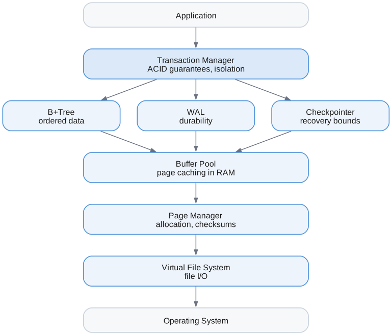
Chapters
Storage Engine
- Virtual File System - Abstracting file I/O for portability and testing
- Portable Databases - Serializing to bytes, and running with no files at all
- Page Manager - Fixed-size pages, allocation, and checksums
- Buffer Pool - Caching pages in memory with eviction
- B+Tree - Ordered key-value storage with efficient lookups
Durability & Transactions
- Write-Ahead Log - Durability through logging before data changes
- Transaction Manager - ACID transactions with begin/commit/abort
- Checkpointing - Bounding recovery time by flushing dirty pages
- Recovery - ARIES-style crash recovery with redo/undo
Data Model
- Graph Storage - Nodes, edges, labels, and properties
- Durable Streams - Transactional event records and semantic graph changes
Search Indexes
- Vector Search - HNSW approximate nearest neighbor search
- Full-Text Search - BM25-scored inverted index, per-property declarations, and search as an access path
Query System
- Query Execution - Volcano iterator model, operators, and planning
Design Principles
Direct Page Manipulation
We don't deserialize pages into objects. Instead, we read/write bytes directly in page buffers. This is "zero-copy" - no intermediate representations, no serialization overhead.
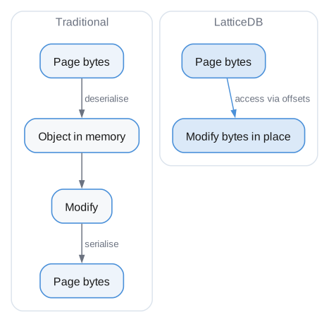
Everything is Pages
The entire database is built on fixed-size pages (4KB by default):
- B+Tree nodes are pages
- Large B+Tree values spill into linked overflow pages
- WAL frames are pages
- The file header is a page
- Free list entries are pages
This uniformity simplifies the system - one caching layer, one I/O path, one checksum format.
Durability Through WAL
Changes are logged before being applied. This means:
- Commit = log is on disk (fast, sequential write)
- Actual data pages can be written lazily
- Crash recovery replays the log
Simple Concurrency Model
Each page has a reader-writer latch. Multiple readers OR one writer. No complex lock hierarchies - simplicity over maximum concurrency.
Virtual File System (VFS)
What It Is
The Virtual File System is an abstraction layer over file I/O operations. Instead of calling OS functions directly, all file operations go through a VFS interface.
Why We Need It
1. Databases that are not files
The most visible thing this buys is databases with nothing underneath them. Open
:memory: and the engine runs against a filesystem held in RAM:
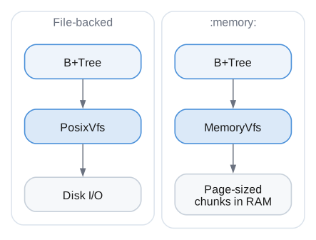
Everything above the interface is unchanged. The B+Tree, the buffer pool, the write-ahead log, and recovery all run exactly as they do against a disk, because none of them knows the difference. That is why in-memory support was a new backend rather than a second path through the engine.
Tests get the same benefit, and run without touching a disk.
2. Portability
Different operating systems have different file APIs:
- Linux:
pread,pwrite,fsync - Windows:
ReadFile,WriteFile,FlushFileBuffers - Embedded: Custom flash drivers
The VFS hides these differences. We implement one VFS per platform, and the rest of the database doesn't care.
3. Injection of Failures
For testing crash recovery, we need to simulate failures:
const FaultyVfs = struct {
inner: Vfs,
fail_after_n_writes: usize,
write_count: usize,
pub fn write(self: *Self, offset: u64, data: []const u8) !void {
self.write_count += 1;
if (self.write_count > self.fail_after_n_writes) {
return error.SimulatedCrash;
}
return self.inner.write(offset, data);
}
};
The Interface
File Operations
pub const File = struct {
ptr: *anyopaque,
vtable: *const VTable,
pub const VTable = struct {
read: fn(ptr, offset: u64, buf: []u8) Error!usize,
write: fn(ptr, offset: u64, data: []const u8) Error!void,
sync: fn(ptr) Error!void,
size: fn(ptr) Error!u64,
close: fn(ptr) void,
truncate: fn(ptr, size: u64) Error!void,
};
// Convenience methods that call vtable
pub fn read(self: File, offset: u64, buf: []u8) !usize {
return self.vtable.read(self.ptr, offset, buf);
}
// ... etc
};
VFS Operations
pub const Vfs = struct {
ptr: *anyopaque,
vtable: *const VTable,
pub const VTable = struct {
open: fn(ptr, path: []const u8, flags: OpenFlags) Error!File,
delete: fn(ptr, path: []const u8) Error!void,
exists: fn(ptr, path: []const u8) bool,
};
};
Open Flags
pub const OpenFlags = struct {
read: bool = true, // Open for reading
write: bool = false, // Open for writing
create: bool = false, // Create if doesn't exist
exclusive: bool = false, // Fail if exists (with create)
};
Key Operations
Positioned Read/Write
Unlike streaming I/O, we use positioned reads and writes:
// Read 4096 bytes starting at byte offset 8192
const bytes_read = try file.read(8192, buffer[0..4096]);
// Write 4096 bytes starting at byte offset 8192
try file.write(8192, data[0..4096]);
This maps directly to page-based access:
- Page 0 is at offset 0
- Page 1 is at offset 4096
- Page N is at offset N * 4096
Sync (fsync)
The most important operation for durability:
try file.sync();
This forces all pending writes to physical storage. Without it, data might sit in OS buffers and be lost on power failure.
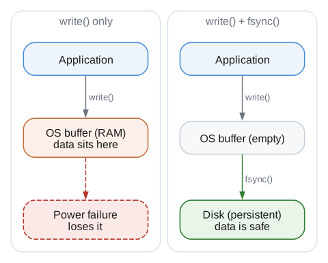
The POSIX Implementation
For Unix-like systems (Linux, macOS):
pub const PosixVfs = struct {
allocator: Allocator,
pub fn open(self: *Self, path: []const u8, flags: OpenFlags) !File {
var posix_flags: u32 = 0;
if (flags.read and flags.write) {
posix_flags |= O_RDWR;
} else if (flags.write) {
posix_flags |= O_WRONLY;
} else {
posix_flags |= O_RDONLY;
}
if (flags.create) posix_flags |= O_CREAT;
if (flags.exclusive) posix_flags |= O_EXCL;
const fd = try std.posix.open(path, posix_flags, 0o644);
// ... wrap in File struct
}
};
Read Implementation
Uses pread for positioned reading (thread-safe, no seeking):
fn read(self: *PosixFile, offset: u64, buf: []u8) !usize {
return std.posix.pread(self.fd, buf, offset);
}
Write Implementation
Uses pwrite for positioned writing:
fn write(self: *PosixFile, offset: u64, data: []const u8) !void {
var written: usize = 0;
while (written < data.len) {
const n = try std.posix.pwrite(self.fd, data[written..], offset + written);
if (n == 0) return error.DiskFull;
written += n;
}
}
Sync Implementation
fn sync(self: *PosixFile) !void {
try std.posix.fsync(self.fd);
}
The Memory Implementation
MemoryVfs holds files in RAM. It backs :memory: databases and databases
opened from bytes, and it is a real backend rather than a testing convenience.
Files are chunks, not one buffer
A file is a list of page-sized pieces:
const Chunk = union(enum) {
borrowed: []const u8,
owned: []u8,
};
The obvious implementation is one growing buffer, and it is the wrong one. A growing buffer has to be reallocated as the file extends, and a reallocation moves every byte to a new address. Anything holding a slice from before that moment is left pointing at freed memory.
That matters because lending slices is the point. A database opened from a caller's bytes can point at them instead of copying, which halves what loading costs. That is only possible if addresses are stable, so chunks came first and the lending was built on top.
Copy-on-write
A chunk either owns its bytes or borrows them from whoever handed them over. Writing to a borrowed chunk copies it first, at page granularity.
So a database loaded from a blob starts out borrowing all of itself, and only the pages actually modified become private copies. Reading a database and changing a little of it keeps one copy of nearly all of it, and the caller's buffer is never modified.
Locking is a no-op
Every lock succeeds. A lock exists to keep a second process off a database, and no other process can reach memory this one owns. That is a decision rather than an omission: file-backed databases take a real lock and refuse a second opener, and this backend declines to pretend there is anything to exclude.
What it costs
Peak memory is the database plus the buffer pool, and the pool is a small constant here — see Buffer Pool for why a cache barely matters when the storage underneath it is already RAM.
100 nodes | database 240 KB | pool 256 KB | 2.62x
4000 nodes | database 7416 KB | pool 256 KB | 1.04x
10000 nodes | database 18432 KB | pool 256 KB | 1.01x
The overhead at small sizes is mostly the write-ahead log, which is a second file in the same backend. It shrinks as automatic checkpointing truncates it, which is why the ratio falls rather than rises as the database grows.
The log stays enabled in memory, incidentally, and that is worth knowing. Turning
it off looks free — a process holding the only copy of a database loses everything
when it dies anyway — but transactions are built on it, so a database without a log
has no BEGIN, no rollback, and no multi-statement atomicity.
Error Handling
VFS operations can fail in various ways:
pub const VfsError = error{
FileNotFound, // Path doesn't exist
PermissionDenied, // No access rights
DiskFull, // No space left
IoError, // Hardware failure
FileLocked, // Another process has it
InvalidPath, // Bad path string
AlreadyExists, // Exclusive create failed
};
These are translated from OS-specific error codes:
fn mapPosixError(err: std.posix.Error) VfsError {
return switch (err) {
.ENOENT => VfsError.FileNotFound,
.EACCES, .EPERM => VfsError.PermissionDenied,
.ENOSPC => VfsError.DiskFull,
.EIO => VfsError.IoError,
// ...
};
}
Usage Pattern
// Create VFS
var posix_vfs = PosixVfs.init(allocator);
const vfs = posix_vfs.vfs(); // Get interface
// Open file
const file = try vfs.open("database.db", .{
.read = true,
.write = true,
.create = true,
});
defer file.close();
// Read page 5
var buf: [4096]u8 = undefined;
_ = try file.read(5 * 4096, &buf);
// Modify and write back
buf[0] = 42;
try file.write(5 * 4096, &buf);
// Ensure durability
try file.sync();
Why Not Just Use std.fs?
Zig's standard library has file operations, but:
- No positioned I/O -
std.fs.Fileuses streaming with seek, which isn't thread-safe - No vtable pattern - Can't swap implementations
- Different error types - We want database-specific errors
The VFS is a thin layer, but it gives us control where we need it.
Portable Databases
What It Is
A LatticeDB database can be handed around as a block of bytes, and it can run with no files behind it at all. Those are two features and one idea: a database is a single file, and the engine reaches that file through an interface it does not control.
This chapter is about how that works and why it was built this way.
Why one file matters
The same request — "let me keep many small databases in object storage and pull one down when I need it" — has been made of several embedded graph databases. For most of them it is hard, because a database is a catalog, a set of index files, a data file, and a log. Serializing means inventing a container format for all of them and keeping it in step with the engine as both change.
Here, serializing a database is reading its file. That is not a clever trick and there is no format to maintain; it falls out of the storage layout. It is the clearest practical argument for the single-file design, which otherwise looks like a mere convenience.
Serializing
serialize does two things:
_ = try self.quiesceForCopy(); // fold everything pending into the file
// ...then read the file
The first step is the interesting one. At any moment part of a database lives somewhere other than its file: dirty pages sit in the buffer pool, committed changes sit in the write-ahead log, and the vector index keeps state in memory until asked to persist it. Copying the file without settling all of that gives you something that opens and is then subtly wrong.
So quiescing persists the vector index, writes the tree roots, and runs a .full
checkpoint, which flushes dirty pages into the file and leaves the log alone. The
result is a file that needs no log beside it — which is exactly what somebody
uploading to a bucket wants, since they are going to upload one object.
backup performs the same step, and the two share it rather than keeping separate
copies that would drift apart.
Why it refuses during a transaction
serialize returns an error if a transaction is open. A copy taken while writes
land underneath it is torn in a way nothing downstream can detect: the bytes are
individually valid, the pages pass their checksums, and the structure is
inconsistent. Failing at the point of the mistake is the only place the problem is
visible.
Why deserialize validates
Opening a zero-length file is how a database gets created. So bytes that are empty
or truncated, written out and opened, would quietly become a brand new empty
database — and report success. deserialize therefore checks the length and magic
number before it does anything with the bytes.
This matters because the obvious failure in this workflow is a partial download.
Running without files
Every byte the storage layer moves goes through the VFS interface.
Swapping the implementation is therefore enough to give a database with nothing
underneath it, and :memory: does exactly that.
Nothing above the interface changes. The B+Tree, buffer pool, log, and recovery all run as they always do, because none of them can tell the difference. That sameness is the entire reason the feature was cheap, and it is worth protecting: the tempting optimizations in this area are mostly ones that would make the in-memory path structurally different, and each would buy a little memory in exchange for a second code path to keep correct.
Why :memory: is a path and not an option
Every binding already accepts a path string and passes it through to the C API. A magic path therefore works everywhere the moment the engine recognises it — Python, TypeScript, Go, C, and the command line — with no binding changes at all.
An option would have meant a new field, so a new versioned C struct, so a new entry point, so FFI declarations and public option types and documentation in four bindings, for exactly the same capability. The cost of the magic string is that it is a magic string.
Opening :memory: also implies creating it, since there is never a previous
in-memory database to find. Requiring create would have been a formality every
caller had to remember, which would have undone the point.
Why the log stays on
Turning the write-ahead log off in memory looks free. A log exists so a crash cannot lose committed data, and a process holding the only copy of a database in its own heap loses everything when it dies regardless.
That reasoning does not survive contact with the code. Transactions are built on
the log, so a database without one returns TransactionsNotEnabled from
beginTransaction: no rollback, no multi-statement atomicity, none of it. That is
a much larger hole than the allocations it saves, and it would make in-memory
databases quietly less capable than file-backed ones in a way nobody would expect.
The log becomes a second file in the same memory backend, bounded by automatic checkpointing.
Why locks always succeed
A file-backed database takes a lock and refuses a second opener, because two processes writing one file corrupt it. No other process can reach memory this one owns, so there is nothing to exclude, and every lock request in the memory backend succeeds.
That is a decision rather than an omission, which is worth stating plainly given the file-backed behaviour is the opposite.
What it costs
100 nodes | database 240 KB | pool 256 KB | total 628 KB | 2.62x
1000 nodes | database 1896 KB | pool 256 KB | total 3412 KB | 1.80x
4000 nodes | database 7416 KB | pool 256 KB | total 7676 KB | 1.04x
10000 nodes | database 18432 KB | pool 256 KB | total 18692 KB | 1.01x
Two things are worth reading out of that table.
The buffer pool is a small constant rather than a fraction of the data, because a cache stops earning its keep when the storage underneath it is already RAM. See Buffer Pool for the measurement behind that.
And the overhead at small sizes is not duplication, it is the write-ahead log living as a second file in the same backend. That is why the ratio falls as the database grows rather than rising: checkpointing truncates the log, and the fixed costs stop mattering.
Loading without a second copy
By default deserialize copies the caller's bytes. It can instead point at them,
which halves what loading costs.
The memory backend stores a file as page-sized chunks, and a chunk either owns its bytes or borrows them:
const Chunk = union(enum) {
borrowed: []const u8,
owned: []u8,
};
Writing to a borrowed chunk copies it first. A database loaded this way starts out borrowing all of itself and only the pages actually modified become private, so reading a database and editing a little of it keeps one copy of nearly all of it. The caller's buffer is never written to.
Why chunks, not one buffer
One growing buffer is the obvious layout and the wrong one. Growing it means reallocating, reallocating moves every byte, and anything holding a slice from before that moment is left pointing at freed memory. Lending slices is the whole point, so stable addresses had to come first.
Why some languages cannot borrow
Python and TypeScript can: the binding keeps a reference to the buffer on the wrapper object, and the collector cannot take it.
Go cannot, and this is a language rule rather than a gap in the binding. Its own
documentation says C code may not keep a copy of a Go pointer after the call
returns, and that slices cannot be pinned to work around it. Java cannot either,
for a different reason: pinning a byte[] for the lifetime of a database would
hold up the collector for exactly that long.
So there are two entry points and each language uses the one its rules allow. The copy happens inside the engine, so the bindings that must copy do not implement anything themselves.
What was considered and rejected
Frames borrowing from the memory backend. The buffer pool could point at pages in the memory backend for clean pages and copy on first write. This was the original plan for reducing duplication, and the measurements above closed it: the pool is a constant 256 KB, so there is nothing material left to save, and the change would add a new state — "this frame might not own its bytes" — to the structure that pinning, latching, and dirty tracking all run through, on every read and write in the engine.
Making the pool the storage. For an in-memory database the pool could be the file, with nothing ever evicted since there is nowhere to evict to. That gives exactly one copy by construction. It is rejected because it makes the in-memory path structurally different from the file path, and that sameness is why this works at all.
Related
- Virtual File System — the interface all of this rests on
- Buffer Pool — why the cache is sized differently here
- Backup and Replication — how to use it
Page Manager
What It Is
The Page Manager handles the lowest level of database storage: fixed-size pages. It manages the database file structure, page allocation/deallocation, and data integrity through checksums.
Why Fixed-Size Pages?
Simplicity
Every piece of data lives in a 4KB page. This uniformity simplifies everything:

To read page N: offset = N * 4096
Alignment with Hardware
- SSD pages: Modern SSDs have 4KB or 8KB internal pages
- OS pages: Most operating systems use 4KB virtual memory pages
- Disk sectors: Traditional HDDs use 512B or 4KB sectors
4KB aligns well with all of these, enabling:
- Direct I/O (bypassing OS cache)
- Atomic writes on some hardware
- Efficient memory mapping
Efficient Caching
Fixed-size pages make the buffer pool trivial - every frame is the same size, no fragmentation.
File Structure
Page 0: File Header
The first page is special - it contains metadata about the database:
| Offset | Size | Field |
|---|---|---|
| 0–3 | 4 B | Magic number — 0x4C415454 ("LATT") |
| 4–5 | 2 B | Format version |
| 6–7 | 2 B | Minimum reader version |
| 8–11 | 4 B | Page size (4096) |
| 12–15 | 4 B | Freelist head page |
| 16–23 | 8 B | Created timestamp |
| 24–31 | 8 B | Modified timestamp |
| 32–47 | 16 B | File UUID |
| 48 → | — | Reserved / padding |
Key fields:
- Magic number: Identifies this as a Lattice database file. Opening a random file will fail fast.
- Format version: Allows future changes to the format
- Freelist head: Points to the first free page (for allocation)
- File UUID: Unique identifier, used to match WAL files
Data Pages
Every other page starts with a common header:
| Offset | Size | Field |
|---|---|---|
| 0–3 | 4 B | Checksum — CRC32 of bytes 8–4095 |
| 4 | 1 B | Page type — btree_internal, btree_leaf, and so on |
| 5 | 1 B | Flags |
| 6–7 | 2 B | Reserved |
| 8–4095 | 4088 B | Page-specific data |
Page Types
pub const PageType = enum(u8) {
free = 0, // Unallocated, on freelist
btree_internal = 1, // B+Tree internal node
btree_leaf = 2, // B+Tree leaf node
overflow = 3, // Large value overflow
freelist = 4, // Freelist continuation
};
Page Allocation
The Freelist
Free pages are linked together in a freelist:

Allocating a Page
pub fn allocatePage(self: *Self) !PageId {
// 1. Try freelist first
if (self.header.freelist_page != NULL_PAGE) {
return self.allocateFromFreelist();
}
// 2. Allocate at end of file
const page_id = self.pageCount();
// 3. Extend file with zeroed page
var zeros: [4096]u8 = [_]u8{0} ** 4096;
const header: *PageHeader = @ptrCast(&zeros);
header.* = PageHeader.init(.free);
try self.file.write(page_id * 4096, &zeros);
return page_id;
}
Allocating from Freelist
fn allocateFromFreelist(self: *Self) !PageId {
const page_id = self.header.freelist_page;
// Read the free page to get next pointer
var buf: [4096]u8 = undefined;
try self.readPageRaw(page_id, &buf);
// Next pointer is stored after the 8-byte header
const next_free = std.mem.readInt(u32, buf[8..12], .little);
// Update freelist head
self.header.freelist_page = next_free;
try self.writeHeader();
return page_id;
}
Freeing a Page
pub fn freePage(self: *Self, page_id: PageId) !void {
// 1. Can't free the header page
if (page_id == 0) return error.InvalidPageId;
// 2. Set up page as free, pointing to current freelist head
var buf: [4096]u8 = [_]u8{0} ** 4096;
const header: *PageHeader = @ptrCast(&buf);
header.* = PageHeader.init(.free);
// Store old freelist head as next pointer
std.mem.writeInt(u32, buf[8..12], self.header.freelist_page, .little);
// 3. Calculate checksum and write
header.checksum = calculateChecksum(buf[8..]);
try self.file.write(page_id * 4096, &buf);
// 4. Update freelist head to this page
self.header.freelist_page = page_id;
try self.writeHeader();
}
This is a LIFO (stack) freelist - last freed is first allocated. Simple and efficient.
Physical Tail Reclamation
Normal allocation reuses freelist pages without moving live pages, so file size
does not need to grow again after deletes. To return space to the operating
system, lattice compact <path> flushes and evicts the buffer pool, rebuilds
the retained freelist, persists a head that excludes tail pages, and truncates
the contiguous free run at physical EOF. Live pages and logical IDs never move.
The header is synced before truncation. A crash between those steps can leave temporarily unreclaimed free pages, but cannot leave a freelist pointer beyond the new end of the file.
Checksums
Every page has a CRC32 checksum that covers bytes 8-4095 (everything after the checksum field itself).
Why Checksums?
- Detect corruption: Hardware failures, cosmic rays, bugs
- Detect torn writes: Partial page writes from crashes
- Validate reads: Catch errors before using bad data
Checksum Calculation
pub fn calculateChecksum(data: []const u8) u32 {
var crc = std.hash.Crc32.init();
crc.update(data);
return crc.final();
}
Writing with Checksum
pub fn writePage(self: *Self, page_id: PageId, buf: []u8) !void {
// Calculate checksum of everything after the checksum field
const header: *PageHeader = @ptrCast(buf.ptr);
header.checksum = calculateChecksum(buf[8..]);
// Write to disk
try self.file.write(page_id * 4096, buf);
}
Reading with Verification
pub fn readPage(self: *Self, page_id: PageId, buf: []u8) !void {
try self.file.read(page_id * 4096, buf);
// Verify checksum
const header: *const PageHeader = @ptrCast(buf.ptr);
const expected = calculateChecksum(buf[8..]);
if (header.checksum != expected and header.checksum != 0) {
return error.ChecksumMismatch;
}
}
Note: Checksum of 0 is allowed for newly allocated pages that haven't been written yet.
Read-Only Mode
The Page Manager supports opening databases read-only:
var pm = try PageManager.init(allocator, vfs, "db.file", .{
.read_only = true,
});
// This fails:
_ = try pm.allocatePage(); // error.PermissionDenied
try pm.writePage(1, &buf); // error.PermissionDenied
Useful for:
- Backup tools
- Read replicas
- Forensic analysis
Error Handling
pub const PageManagerError = error{
InvalidHeader, // File header is malformed
InvalidMagic, // Not a Lattice database file
VersionTooNew, // File created by newer version
ChecksumMismatch, // Data corruption detected
InvalidPageId, // Page ID out of range
PageNotAllocated, // Accessing unallocated page
IoError, // Underlying I/O failed
PermissionDenied, // Write to read-only database
FileNotFound, // Database file doesn't exist
DiskFull, // No space for new pages
};
Thread Safety
The Page Manager itself is NOT thread-safe. Each operation directly touches the file. In a multi-threaded context, the Buffer Pool provides thread-safe access by:
- Caching pages in memory
- Using latches (reader-writer locks) per page
- Serializing writes through its own mutex
Usage Pattern
// Open or create database
var pm = try PageManager.init(allocator, vfs, "my.db", .{
.create = true,
.page_size = 4096,
});
defer pm.deinit();
// Allocate a page
const page_id = try pm.allocatePage();
// Write data
var buf: [4096]u8 align(4096) = undefined;
const header: *PageHeader = @ptrCast(&buf);
header.* = PageHeader.init(.btree_leaf);
// ... fill in page data ...
try pm.writePage(page_id, &buf);
// Read it back
var read_buf: [4096]u8 align(4096) = undefined;
try pm.readPage(page_id, &read_buf);
// Free the page
try pm.freePage(page_id);
// Ensure durability
try pm.sync();
Key Design Decisions
Fixed 4KB Pages
Chosen for hardware alignment. Could be made configurable (stored in header), but 4KB works well for most cases.
Freelist in Pages
The freelist uses the free pages themselves for storage. No external data structure needed. Elegant and space-efficient.
Checksum After Header
Checksum doesn't cover itself (circular dependency). By placing checksum first, we can compute it over the rest of the page in one pass.
No Internal Fragmentation Tracking
We don't track free space within pages - that's the responsibility of higher layers (B+Tree). The Page Manager only deals with whole pages.
Buffer Pool
What It Is
The Buffer Pool is a cache that keeps frequently accessed pages in memory. Instead of reading from disk every time, we check the buffer pool first.
The Problem It Solves
Disk I/O is slow:
| Operation | Typical latency |
|---|---|
| CPU instruction | ~1 ns |
| RAM access | ~100 ns |
| SSD read | ~100,000 ns (100 µs) |
| HDD read | ~10,000,000 ns (10 ms) |
RAM is 1,000-100,000x faster than disk. If we can keep hot pages in RAM, performance improves dramatically.
Architecture
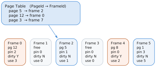
The Frame
Each frame holds one page:
pub const BufferFrame = struct {
page_id: PageId, // Which page is here (0 = empty)
data: []align(4096) u8, // The actual 4KB page data
pin_count: atomic(u32), // Reference count
dirty: bool, // Modified since read?
usage_count: u8, // For Clock eviction
latch: RwLatch, // Reader-writer lock
};
Pin Count
The pin count is a reference count:
| Call | Effect | Meaning |
|---|---|---|
fetchPage() | pin_count += 1 | I am using this page |
unpinPage() | pin_count -= 1 | I am done with this page |
| Pin count | Consequence |
|---|---|
> 0 | Page is in use and cannot be evicted |
= 0 | Page may be evicted if a frame is needed |
Dirty Flag
| Event | Dirty flag | Meaning |
|---|---|---|
| Read page | false | Frame matches disk |
| Modify page | true | Frame differs from disk |
| Write to disk | false | Frame matches disk again |
Dirty pages MUST be written to disk before eviction. Otherwise we lose data!
Reader-Writer Latch
Multiple readers OR one writer
Read latch: "I'm reading, others can read too"
Write latch: "I'm modifying, exclusive access"
Fetching a Page
pub fn fetchPage(self: *Self, page_id: PageId, mode: LatchMode) !*BufferFrame {
self.mutex.lock();
defer self.mutex.unlock();
// 1. Check if already in buffer pool
if (self.page_table.get(page_id)) |frame_id| {
const frame = &self.frames[frame_id];
frame.pin_count.fetchAdd(1, .monotonic);
frame.usage_count = @min(frame.usage_count + 1, 255);
acquireLatch(frame, mode);
return frame;
}
// 2. Not in pool - need to load from disk
const frame = try self.findVictimFrame();
// 3. If victim is dirty, flush it first
if (frame.dirty) {
try self.pm.writePage(frame.page_id, frame.data);
frame.dirty = false;
}
// 4. Update page table
if (frame.page_id != NULL_PAGE) {
self.page_table.remove(frame.page_id);
}
self.page_table.put(page_id, frame_id);
// 5. Read page from disk
try self.pm.readPage(page_id, frame.data);
// 6. Set up frame
frame.page_id = page_id;
frame.pin_count.store(1, .monotonic);
frame.dirty = false;
frame.usage_count = 1;
acquireLatch(frame, mode);
return frame;
}
The Clock Eviction Algorithm
When the buffer pool is full, we need to evict a page to make room. We use the Clock algorithm (also called "second chance").
Why Clock?
- LRU (Least Recently Used) is optimal but expensive - requires updating timestamps on every access
- Clock approximates LRU cheaply using a usage bit
How It Works
Imagine the frames arranged in a circle with a clock hand:
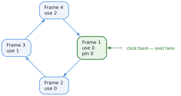
To find a victim:
fn findVictimFrame(self: *Self) !*BufferFrame {
// Try free list first
if (self.free_list.pop()) |frame_id| {
return &self.frames[frame_id];
}
// Clock sweep
var attempts: usize = 0;
while (attempts < self.frame_count * 2) {
const frame = &self.frames[self.clock_hand];
// Move hand
self.clock_hand = (self.clock_hand + 1) % self.frame_count;
attempts += 1;
// Skip pinned pages
if (frame.pin_count.load(.monotonic) > 0) {
continue;
}
// Second chance: if used recently, clear and skip
if (frame.usage_count > 0) {
frame.usage_count -= 1;
continue;
}
// Found victim!
return frame;
}
return error.BufferPoolFull; // All pages pinned
}
The key insight: Usage count gives pages a "second chance". Recently used pages survive one clock sweep. Only pages that haven't been used in a full rotation get evicted.
Unpinning Pages
When done with a page:
pub fn unpinPage(self: *Self, frame: *BufferFrame, dirty: bool) void {
// Release latch
frame.latch.release();
// Mark dirty if modified
if (dirty) {
frame.dirty = true;
}
// Decrement pin count
_ = frame.pin_count.fetchSub(1, .monotonic);
}
Always unpin! Failure to unpin causes:
- Pages stuck in memory forever
- Buffer pool eventually fills with pinned pages
BufferPoolFullerrors
Flushing Pages
Writing dirty pages to disk:
// Flush one page
pub fn flushPage(self: *Self, page_id: PageId) !void {
const frame = self.getFrame(page_id) orelse return;
if (frame.dirty) {
try self.pm.writePage(frame.page_id, frame.data);
frame.dirty = false;
}
}
// Flush all dirty pages
pub fn flushAll(self: *Self) !void {
for (self.frames) |*frame| {
if (frame.page_id != NULL_PAGE and frame.dirty) {
try self.pm.writePage(frame.page_id, frame.data);
frame.dirty = false;
}
}
}
Thread Safety
The buffer pool is thread-safe:
- Mutex protects page_table, free_list, clock_hand
- Per-frame latches protect page data
- Atomic pin_count for safe reference counting
| Step | Thread 1 — fetchPage(5) | Thread 2 — fetchPage(5) |
|---|---|---|
| 1 | mutex.lock() | mutex.lock() — blocked |
| 2 | look up page 5 | waiting |
| 3 | pin_count++ | waiting |
| 4 | mutex.unlock() | mutex.lock() — acquired |
| 5 | frame.latch.read() | look up page 5 — found |
| 6 | read data | pin_count++ |
| 7 | read data | mutex.unlock() |
| 8 | read data | frame.latch.read() |
| 9 | unpinPage() | read data |
| 10 | — | unpinPage() |
The page table mutex is held only long enough to find the frame and bump the pin count. Reading the page data happens under the per-frame latch, so two readers of the same page overlap rather than serialising.
Multiple threads can read the same page concurrently (shared latch).
Memory Alignment
Page buffers are 4KB-aligned:
const data = try allocator.alignedAlloc(u8, 4096, page_size);
Why?
- Direct I/O: Some systems require aligned buffers for O_DIRECT
- SIMD: Aligned data enables vectorized operations
- Cache lines: Better CPU cache utilization
Sizing the Buffer Pool
// 64MB buffer pool = 16,384 pages
var bp = try BufferPool.init(allocator, &pm, 64 * 1024 * 1024);
Guidelines:
- More is better (to a point)
- Working set: Should fit frequently accessed pages
- Available RAM: Leave room for OS and other processes
- Typical: 25-75% of available RAM
In-memory databases are different
All of the above assumes there is a disk to avoid. When the storage underneath is
already RAM — a :memory: database, or one opened from bytes — a cache miss costs
a copy from one part of memory to another rather than a trip to a device, so the
pool stops being the difference between fast and slow.
Measured on a fourteen megabyte in-memory database, twelve full scans took 9.2 seconds against a 256 KB pool and 9.9 against a 32 MB one. A hundred and twenty times the memory bought nothing.
So an in-memory database gets a small fixed pool rather than a fraction of the data. That keeps peak memory close to the size of the database itself, which matters when the point of the feature is holding many small databases at once.
The floor is a correctness requirement, not a tuning choice. When the clock
sweep finds no evictable frame the pool returns BufferPoolFull, and that surfaces
as a failed query rather than a slow one. The pool must always have room for the
largest set of pages pinned simultaneously.
That number was measured rather than guessed, since guessing it trades memory against query failures. Pools from four frames upward were run through a deep variable-length traversal, a filtered scan, a full-text search, and a bulk write over a fifteen-hundred node graph. Four frames completed all of it — the engine does not hold many pages pinned at once. The floor sits at sixty-four, sixteen times that, because the measurement was single threaded and concurrent readers each pin pages of their own.
Usage Pattern
var bp = try BufferPool.init(allocator, &pm, pool_size);
defer bp.deinit(); // Flushes dirty pages
// Read a page
const frame = try bp.fetchPage(page_id, .shared);
defer bp.unpinPage(frame, false);
const value = readValueFromPage(frame.data);
// Modify a page
const frame = try bp.fetchPage(page_id, .exclusive);
defer bp.unpinPage(frame, true); // true = dirty
modifyPage(frame.data);
Key Invariants
- Pin before access: Never access page data without pinning
- Unpin when done: Every fetchPage must have matching unpinPage
- Mark dirty: If you modified the page, set dirty=true when unpinning
- Flush before close: deinit() flushes, or call flushAll() explicitly
B+Tree
What It Is
A B+Tree is a self-balancing tree structure optimized for disk-based storage. It provides O(log N) lookups, inserts, and deletes, with efficient range scans.
Why B+Tree?
The Problem with Binary Trees
A binary search tree with 1 million entries is ~20 levels deep (log2(1M) ≈ 20). Each level requires a disk read. That's 20 disk reads per lookup!
B+Tree: Wide and Shallow
A B+Tree has many keys per node (hundreds), making it very shallow:
Binary Tree (1M entries): B+Tree (1M entries):
depth ~20 depth ~3
○ ○
/ \ / | \
○ ○ ○ ○ ○
/\ /\ / | \ / | \ / | \
○ ○ ○ ○ ○ ○ ○ ○ ○ ○ ○ ○
... (20 levels) (leaf level)
20 disk reads 3 disk reads!
With 100 keys per node: log100(1M) ≈ 3 levels.
Data Only in Leaves
B+Trees store all data in leaf nodes. Internal nodes only contain keys for routing:
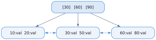
Our Implementation: Direct Page Manipulation
We don't create "node objects" in memory. Instead, we read/write bytes directly in page buffers. The "node" is just a lens over page bytes.
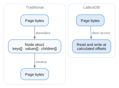
No intermediate objects. No serialization overhead.
Page Layout
Leaf Node
Leaf pages are slotted pages. The header and slot array grow forward from byte 0; entry bytes grow backward from byte 4095; free space is whatever remains in the middle.
| Offset | Size | Field |
|---|---|---|
| 0–7 | 8 B | Page header — checksum, type (leaf), flags |
| 8–9 | 2 B | Entry count (u16) |
| 10–11 | 2 B | Flags (u16) |
| 12–15 | 4 B | Next leaf page (u32) |
| 16–19 | 4 B | Previous leaf page (u32) |
| 20 → | 2 B each | Slot array — one entry_offset (u16) per entry, growing forward |
| ← 4095 | variable | Entries, growing backward: [key_len][value_len][key][value or overflow descriptor] |
Variable-length entries: Keys and values are stored at the end of the page, growing downward from high offsets. Slots at the front point to the entry records.
Large values are stored through generic B+Tree overflow records. A leaf entry uses the normal key bytes plus a compact overflow descriptor; the descriptor contains the total value length, first overflow page, page count, checksum, and a small local prefix. Point reads and range scans materialize the full value transparently, and deletes free the overflow chain.
Values up to 64 MiB are accepted by the B+Tree layer when the key and overflow
descriptor can fit in an empty leaf. Inline-capable values may still be stored
as overflow records when keeping them inline would make future 4 KiB leaf splits
impossible to divide into two valid ordered pages.
Internal Node
Internal pages use the same slotted layout, but each slot carries a child pointer alongside the key offset, and the values are separator keys rather than user data.
| Offset | Size | Field |
|---|---|---|
| 0–7 | 8 B | Page header — checksum, type (internal), flags |
| 8–9 | 2 B | Key count (u16) |
| 10–11 | 2 B | Level (u16; 0 = parent of leaves) |
| 12–15 | 4 B | Rightmost child (u32) |
| 16 → | 6 B each | Slot array — key_offset (u16) plus child_page (u32), growing forward |
| ← 4095 | variable | Separator keys, growing backward |
Point Lookup
Finding a value by key:
pub fn get(self: *Self, key: []const u8) !?[]const u8 {
// 1. Start at root
var page_id = self.root_page;
while (true) {
// 2. Fetch page from buffer pool
const frame = try self.bp.fetchPage(page_id, .shared);
defer self.bp.unpinPage(frame, false);
const page_type = getPageType(frame.data);
if (page_type == .btree_leaf) {
// 3. Binary search in leaf
return LeafNode.search(frame.data, key, self.comparator);
} else {
// 4. Binary search for child pointer, descend
page_id = InternalNode.findChild(frame.data, key, self.comparator);
}
}
}
Example lookup for key "dog":
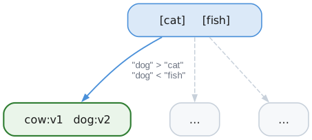
Insertion
Simple Case: Space in Leaf
pub fn insert(self: *Self, key: []const u8, value: []const u8) !void {
// 1. Find the leaf
const leaf_page = try self.findLeaf(key);
// 2. Fetch with exclusive latch
const frame = try self.bp.fetchPage(leaf_page, .exclusive);
defer self.bp.unpinPage(frame, true);
// 3. Prepare either inline bytes or an overflow descriptor
const prepared = try self.prepareStoredValue(key, value);
// 4. Check if the prepared entry fits
if (LeafNode.hasSpace(frame.data, key.len, prepared.value.len)) {
// 5. Insert directly
LeafNode.insert(frame.data, key, prepared.value, self.comparator);
} else {
// 6. Need to split
try self.splitLeafAndInsert(frame, key, prepared);
}
}
Splitting a Leaf
When a leaf is full:
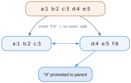
fn splitLeaf(self: *Self, frame: *BufferFrame, key: []const u8, value: []const u8) !void {
// 1. Allocate new page
const new_page = try self.pm.allocatePage();
const new_frame = try self.bp.fetchPage(new_page, .exclusive);
// 2. Find a byte-balanced split point that keeps both leaves valid.
const split_point = try self.chooseLeafSplitPoint(frame.data, key, value);
// 3. Move upper half to new page
LeafNode.moveEntries(frame.data, new_frame.data, split_point, entry_count);
// 4. Insert new key into appropriate page
if (compare(key, split_key) < 0) {
LeafNode.insert(frame.data, key, value);
} else {
LeafNode.insert(new_frame.data, key, value);
}
// 5. Update sibling pointers
LeafNode.setNext(frame.data, new_page);
LeafNode.setPrev(new_frame.data, frame.page_id);
// 6. Get separator key and insert into parent
const separator = LeafNode.getFirstKey(new_frame.data);
try self.insertIntoParent(frame.page_id, separator, new_page);
}
The split point is chosen by serialized byte size, not just entry count. This matters when a leaf mixes small keys with large values: both halves must fit in the configured page size after the new entry is included.
Growing the Tree
When the root splits, we create a new root:
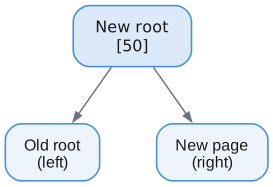
The tree grows at the top, not the bottom. All leaves stay at the same depth.
Range Scan
Thanks to linked leaves, range scans are efficient:
pub fn range(self: *Self, start: ?[]const u8, end: ?[]const u8) !Iterator {
// 1. Find starting leaf
const start_page = if (start) |k|
try self.findLeaf(k)
else
try self.findLeftmostLeaf();
return Iterator{
.btree = self,
.current_page = start_page,
.current_slot = 0,
.end_key = end,
};
}
Iterator walks the leaf chain:
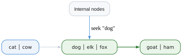
No need to traverse internal nodes for each entry - just follow the links.
Concurrency
We use latch crabbing (simplified):
Lookup (read-only):
1. Latch root (shared)
2. Latch child (shared)
3. Unlatch root
4. Latch grandchild (shared)
5. Unlatch child
... continue to leaf
Insert (may modify):
1. Latch root (exclusive)
2. If child is safe (won't split), latch child and unlatch root
3. Continue down
A "safe" node is one with enough space that it won't split (for insert) or won't underflow (for delete).
The BTree Struct
pub const BTree = struct {
bp: *BufferPool, // Page cache
root_page: PageId, // Current root
comparator: KeyComparator, // For ordering
page_size: u32, // Usually 4096
allocator: Allocator,
// ...methods
};
This is just ~40 bytes of metadata. The actual data lives in pages on disk.
Key Design Decisions
Variable-Length Keys and Values
We store the actual bytes, not fixed-size slots. This supports:
- Short keys efficiently (no wasted space)
- Long keys (up to page size)
- Any binary data
Separator Keys in Internal Nodes
Internal nodes store separator keys, not full key-value pairs. This maximizes fanout (keys per internal node).
Delete Compaction and Leaf Merging
Deletes remove the slot, rebuild the surviving leaf entries contiguously, and free any overflow chain owned by the removed entry. Afterward, adjacent leaves under the same parent are merged whenever their combined payload fits on one page. The redundant leaf is unlinked and returned to the freelist, and a root with only that leaf remaining is collapsed. Space within a surviving leaf is reusable immediately by later inserts or updates, while reclaimed pages are reused by any later database allocation.
When a sparse leaf cannot merge because its sibling is too full, entries are redistributed by stored byte size and the parent separator is updated. Removing a leaf separator can in turn rebalance internal pages: compatible internal siblings absorb their parent separator and merge, while oversized pairs redistribute keys and promote a new separator. Rebalancing propagates to the root, collapsing every now-redundant tree level.
Page-Based, With Explicit Overflow
Each B+Tree node is exactly one page. Large values span linked overflow pages through an explicit descriptor stored in the leaf; ordinary internal and leaf pages remain fixed-size and directly addressable.
Example: Full Insert Sequence
Insert "zebra" into a tree:
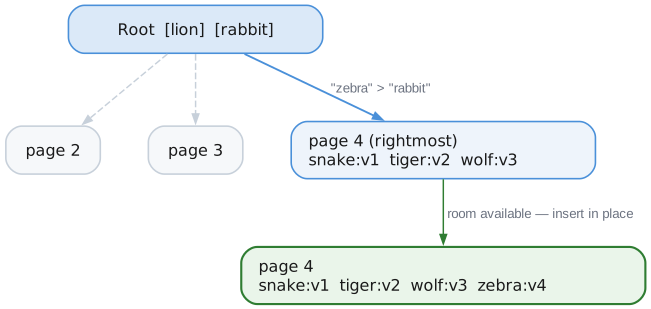
Performance Characteristics
| Operation | Average Case | Worst Case |
|---|---|---|
| Lookup | O(log N) | O(log N) |
| Insert | O(log N) | O(log N) |
| Range(k) | O(log N + k) | O(log N + k) |
Where N is the number of entries and k is the number of entries in range.
Disk I/O per operation: ~3-4 reads for trees up to billions of entries.
Write-Ahead Log (WAL)
The Problem
Imagine you're updating a B+Tree. You need to:
- Modify a leaf page
- Maybe split it (modify parent)
- Maybe split the parent (modify grandparent)
- Update the root
If power fails between steps 2 and 3, your database is corrupted - the tree structure is broken.
Even a single page write isn't safe. A 4KB page write might not be atomic at the hardware level - you could end up with half old data, half new data (a "torn write").
The Insight
Instead of modifying data pages directly, first write a log of what you intend to do. The log is append-only and sequential. Only after the log is safely on disk do you modify the actual data pages.
If you crash:
- Before log write: Nothing happened, no corruption
- After log write, before data write: Replay the log to finish the operation
- After both: Everything is fine
This is the write-ahead rule: log first, then data.
Why Append-Only Sequential Writes Are Special
The WAL relies on a key property: sequential append is much safer than random writes.
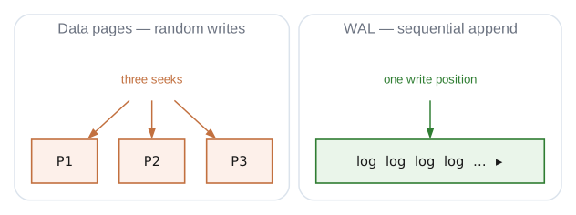
With random writes, the disk head jumps around. A crash can leave any combination of pages in inconsistent states.
With sequential append:
- Only one "frontier" where writing happens
- Everything before the frontier is complete
- Everything after doesn't exist yet
- Much simpler to reason about crash states
The System Primitive: fsync
The WAL's safety depends on one critical system call: fsync (or fdatasync).
write(fd, data, len); // Data goes to OS buffer cache
fsync(fd); // Forces data to physical disk platters
Without fsync, your "written" data might sit in RAM for seconds or minutes. A power failure loses it. fsync is a durability barrier - when it returns, data is on persistent storage.
This is expensive (milliseconds, not microseconds), so we batch multiple records into frames before syncing.
WAL Structure
The WAL file is a 4 KB header followed by a sequence of 4 KB frames.
WAL header (4 KB)
| Field | Purpose |
|---|---|
magic | 0x574C4F47 ("WLOG") |
database_uuid | Binds this WAL to one database file |
frame_count | How many frames have been written |
checkpoint_lsn | Where recovery starts replaying |
checksum | Detects header corruption |
Frame header (32 bytes, at the start of every 4 KB frame)
| Field | Purpose |
|---|---|
frame_number | Position of this frame in the file |
record_count | How many records the frame carries |
data_size | Bytes of the frame actually used |
checksum | CRC32 over the frame's data area |
The remainder of each frame holds records back to back, then unused space. A frame carrying a single-statement transaction might look like this:
| LSN | Record | Transaction |
|---|---|---|
| 1 | TXN_BEGIN | 1 |
| 2 | INSERT (with payload) | 1 |
| 3 | TXN_COMMIT | 1 |
LSN: The Universal Clock
Every record gets a Log Sequence Number (LSN) - a monotonically increasing integer.
LSN 1: TXN_BEGIN (txn 1)
LSN 2: INSERT key="alice" (txn 1)
LSN 3: INSERT key="bob" (txn 1)
LSN 4: TXN_BEGIN (txn 2)
LSN 5: DELETE key="charlie" (txn 2)
LSN 6: TXN_COMMIT (txn 1)
LSN 7: TXN_ABORT (txn 2)
LSN serves multiple purposes:
- Ordering: Total order of all operations
- Recovery point: "Replay from LSN 42"
- Page tracking: Each data page stores the LSN of the last modification
The prev_lsn Chain
Each record stores prev_lsn - the previous LSN for the same transaction:
| LSN | Record | Transaction | prev_lsn |
|---|---|---|---|
| 1 | TXN_BEGIN | 1 | 0 |
| 2 | INSERT | 1 | 1 |
| 3 | INSERT | 2 | 0 |
| 4 | UPDATE | 1 | 2 |
| 5 | TXN_COMMIT | 1 | 4 |
Following prev_lsn from LSN 5 walks transaction 1 backwards — 5 → 4 → 2 → 1 —
skipping LSN 3, which belongs to transaction 2.
This creates a backward chain for each transaction:
Transaction 1: LSN 5 → LSN 4 → LSN 2 → LSN 1
Transaction 2: LSN 3 (just one operation)
Why? Rollback. To abort transaction 1, follow the chain backward, undoing each operation.
Write Flow
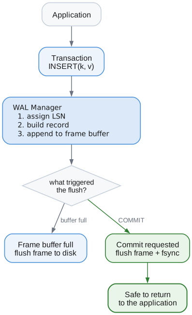
The key insight: we buffer multiple records in memory, only hitting disk when:
- The frame buffer is full (4KB of records accumulated)
- A transaction commits (durability guarantee)
Logical WAL records can be larger than a single frame. Large graph, stream, vector, and
property payloads are fragmented into physical large_fragment records and
reassembled by recovery before redo. The logical payload limit is 64 MiB; a
record above that limit returns ValueTooLarge.
Vector replacements and removals are logical transaction records too. Recovery replays them into the vector index only for committed transactions; an index that cannot replay a vector record causes open to fail rather than return incomplete search results. Open with vector support and the same dimensions as the writer. The initial empty tree pages and out-of-transaction FTS declarations are persisted before writes rely on them. Recovered indexes and their roots are flushed before open returns, so recovery does not require a later clean close to survive.
Commit Protocol
When you call COMMIT:
1. Write TXN_COMMIT record to WAL buffer
2. Flush current frame to disk
3. Call fsync() - WAIT for disk acknowledgment
4. Return "committed" to application
After step 3, even if power fails immediately, the commit record is on disk. Recovery will see the commit and know the transaction succeeded.
If we crash before step 3? The commit record might be lost. Recovery won't see a commit for that transaction, so it will be rolled back. No partial commits ever escape to the application.
Recovery: Redo and Undo
On startup after a crash, we need to:
- Find the end of valid log - Scan frames, verify checksums, find last valid record
- Redo committed transactions - Replay all operations from committed transactions
- Undo uncommitted transactions - Roll back any transaction without a commit record
| LSN | Record | Transaction |
|---|---|---|
| 1 | TXN_BEGIN | 1 |
| 2 | INSERT x=1 | 1 |
| 3 | TXN_BEGIN | 2 |
| 4 | INSERT y=2 | 2 |
| 5 | TXN_COMMIT | 1 |
| 6 | INSERT z=3 | 2 |
The process crashes after LSN 6.
| Transaction | Has TXN_COMMIT? | Recovery action |
|---|---|---|
| 1 | Yes | Redo — x=1 is permanent |
| 2 | No | Undo — y=2 and z=3 are rolled back |
Why Frames?
Why not just append individual records?
Reason 1: Atomicity
A 4KB write is more likely to be atomic than arbitrary-sized writes. Many storage systems guarantee 512-byte or 4KB atomic writes. By aligning to page boundaries, we reduce torn write risk.
Reason 2: Batching
Each fsync is expensive (~1-10ms). By batching records into frames, we amortize the sync cost across many operations.
Reason 3: Checksums
Each frame has a checksum. During recovery, we can detect partial/corrupted frames and stop replay at the right point.
Reason 4: Large logical records
Frames remain page-sized for torn-write detection and batching, but the WAL no longer requires each logical record to fit inside one frame. Fragmentation keeps large transactional property updates on the WAL path without changing the frame format used for normal records.
The Checksum
We use CRC32 to detect corruption:
Every frame stores a CRC32 of its data area in its header:
| Frame region | Contents |
|---|---|
| Header | checksum = 0xABCD1234 |
| Data | [record 1][record 2][record 3] |
On read the checksum is recomputed and compared:
- Read the frame.
- Compute
CRC32(data). - Compare against the stored checksum.
- On mismatch, corruption is detected and replay stops.
This catches:
- Torn writes (partial frame written)
- Bit rot (storage degradation)
- Wrong WAL file (UUID also checked)
The UUID Link
The WAL header stores the database file's UUID:

This prevents accidentally using database A's WAL with database B. The UUID is generated randomly when the database is created.
Record Types
pub const WalRecordType = enum(u8) {
// Transaction control
txn_begin = 0x01,
txn_commit = 0x02,
txn_abort = 0x03,
// Data modifications
insert = 0x10,
update = 0x11,
delete = 0x12,
// Page-level operations
page_write = 0x20,
// Checkpointing
checkpoint_begin = 0x30,
checkpoint_end = 0x31,
// Savepoints
savepoint = 0x40,
savepoint_rollback = 0x41,
// Compensation (for undo during recovery)
clr = 0x50,
};
WalManager API
// Append a record, get back its LSN
const lsn = try wal.appendRecord(.insert, txn_id, prev_lsn, payload);
// Force all buffered records to disk
try wal.sync();
// Iterate records for recovery
var iter = wal.iterate(start_lsn);
while (try iter.next(&buf)) |record| {
// Process record
}
// Update checkpoint position
try wal.setCheckpointLsn(lsn);
Summary
| Concept | Purpose |
|---|---|
| Write-ahead rule | Log before data = crash safety |
| Sequential append | Simpler crash states than random writes |
| fsync | Durability barrier to physical storage |
| LSN | Universal ordering of all operations |
| prev_lsn chain | Enables transaction rollback |
| Frames | Atomic-ish writes + batching |
| Checksums | Detect corruption and torn writes |
| UUID | Match WAL to correct database file |
The WAL transforms the problem from "make random writes atomic" (very hard) to "make sequential append reliable" (much easier).
Transaction Manager
What is a Transaction?
A transaction is a logical unit of work - a group of operations that should either all succeed or all fail together.
| Without transactions | With transactions | |
|---|---|---|
| Step 1 | Debit Alice $100 — succeeds | BEGIN |
| Step 2 | Crash | Debit Alice $100 |
| Step 3 | Credit Bob $100 — never runs | Credit Bob $100 |
| Step 4 | — | COMMIT |
| Result | Alice lost $100 and Bob got nothing | Either both happen or neither does |
The ACID Properties
Transactions guarantee four properties:
| Property | Meaning | How We Achieve It |
|---|---|---|
| Atomicity | All or nothing | WAL + rollback |
| Consistency | Valid state to valid state | Application logic |
| Isolation | Transactions don't interfere | Timestamps + MVCC |
| Durability | Committed = permanent | WAL + fsync |
The Core Data Structures
Transaction (User-Facing Handle)
This is what the application sees:
pub const Transaction = struct {
id: u64, // Unique identifier (1, 2, 3, ...)
state: TxnState, // active, committed, or aborted
mode: TxnMode, // read_only or read_write
isolation: IsolationLevel, // snapshot, read_committed, serializable
start_ts: u64, // When transaction started (for visibility)
commit_ts: u64, // When committed (0 until commit)
};
TxnEntry (Internal State)
The manager keeps more detailed state internally:
const TxnEntry = struct {
txn: Transaction, // The user-facing handle
last_lsn: u64, // LSN of most recent operation
begin_lsn: u64, // LSN of TXN_BEGIN record
savepoints: ArrayList, // Stack of savepoints
undo_log: ArrayList, // Operations to reverse on abort
};
TxnManager (The Coordinator)
pub const TxnManager = struct {
allocator: Allocator,
wal: *WalManager, // For durability
active_txns: HashMap(u64, TxnEntry), // All running transactions
next_txn_id: u64, // Counter for IDs
current_ts: u64, // Global timestamp clock
committed_count: u64, // Statistics
aborted_count: u64,
mutex: Mutex, // Thread safety
};
Transaction Lifecycle
1. BEGIN
When you start a transaction:
- Lock the manager mutex.
- Assign
txn_id = 1. - Assign
start_ts = 1. appendRecord(TXN_BEGIN)— the WAL returnslsn = 1.- Create a
TxnEntrywithlast_lsn = 1. - Store it in
active_txns. - Unlock the mutex.
- Return
Transaction { id = 1, ... }to the caller.
The start_ts is crucial for isolation - it determines what data this transaction can "see".
2. Operations
Each modification goes through logOperation:
- Check
txn.canWrite(). - Look up the
TxnEntry. appendRecord(INSERT, txn_id = 1, prev_lsn = 1, payload = data)—prev_lsnis the entry's currentlast_lsn. The WAL returnslsn = 2.- Update
last_lsn = 2. - Return
lsn = 2to the caller.
Notice how prev_lsn points to the previous operation. This builds a backward chain.
3. COMMIT
Commit makes everything permanent:
- Check that
txn.state == active. appendRecord(TXN_COMMIT, prev_lsn = last_lsn).wal.sync()— this issues thefsync(), and it is the point at which the transaction becomes durable. Everything before this step can still be lost.- Assign
commit_ts. - Set
txn.state = committed. - Remove the entry from
active_txns. - Increment
committed_count. - Return to the caller.
The critical point: We only return success to the application AFTER fsync() completes. This is the durability guarantee.
Graph, vector, FTS, and stream mutations are staged in a transaction overlay until commit. At commit time the database logs the semantic graph state needed for recovery, stages graph changefeed records, flushes the WAL, and then applies the overlay to the base stores. Large property updates avoid carrying both old and new full values in commit-time WAL records when redo does not require both; the changefeed uses summary maps for values that would exceed stream/WAL sizing limits.
4. ABORT
Abort discards everything:
appendRecord(TXN_ABORT).wal.sync().- Set
txn.state = aborted. - Clean up the
TxnEntry. - Remove it from
active_txns. - Return to the caller.
We log TXN_ABORT so that during crash recovery, we know this transaction was intentionally aborted.
The prev_lsn Chain
Every record points back to the previous record from the same transaction. This creates a linked list through the WAL:
| LSN | Record | Transaction | prev_lsn |
|---|---|---|---|
| 1 | TXN_BEGIN | 1 | 0 |
| 2 | INSERT | 1 | 1 |
| 3 | TXN_BEGIN | 2 | 0 |
| 4 | UPDATE | 1 | 2 |
| 5 | DELETE | 2 | 3 |
| 6 | TXN_COMMIT | 1 | 4 |
Following prev_lsn backwards gives each transaction's chain without scanning the
whole log:
- Transaction 1: 6 → 4 → 2 → 1
- Transaction 2: 5 → 3
Why is this useful?
- Rollback: To abort transaction 1, follow 6->4->2->1, undoing each operation
- Recovery: After crash, find uncommitted transactions by following chains
- No scanning: Don't need to scan entire WAL to find a transaction's operations
Savepoints: Partial Rollback
Sometimes you want to undo part of a transaction, not all of it:
BEGIN;
INSERT user Alice; -- LSN 2
SAVEPOINT before_orders; -- Remember this point
INSERT order #1; -- LSN 4
INSERT order #2; -- LSN 5
-- Oops, orders were wrong
ROLLBACK TO before_orders; -- Undo LSN 4, 5
INSERT order #3; -- LSN 7
COMMIT;
How Savepoints Work
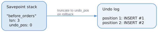
When we rollback to savepoint:
- Find the savepoint by name
- Log
SAVEPOINT_ROLLBACKto WAL - Truncate undo_log to
undo_position - Remove savepoints created after this one
Timestamps and Isolation
Every transaction gets two timestamps:
start_ts: Assigned at BEGIN - determines what data is visible
commit_ts: Assigned at COMMIT - marks when changes become visible to others
Snapshot Isolation Example
| Timestamp | Transaction | Event |
|---|---|---|
| 1 | Txn A | BEGIN — start_ts = 1 |
| 2 | Txn A | INSERT x = 100 |
| 3 | Txn B | BEGIN — start_ts = 3 |
| 4 | Txn A | COMMIT — commit_ts = 4 |
| 5 | Txn B | Reads x |
Txn B began at ts = 3, before Txn A committed at ts = 4, so its snapshot does not
include x = 100 even though the read happens afterwards.
Question: What does Txn B see when it reads x?
With snapshot isolation: Txn B started at ts=3, before Txn A committed at ts=4. So Txn B does NOT see x=100. It sees whatever x was before Txn A.
This is why we track start_ts and commit_ts - they determine visibility.
Read-Only Transactions
Read-only transactions are special:
var txn = try tm.begin(.read_only, .snapshot);
// This fails:
const result = tm.logOperation(&txn, .insert, "data");
// Error: TxnError.ReadOnly
Why have read-only transactions?
- No WAL writes - faster, no disk I/O for reads
- No locks needed - can always proceed
- Never abort due to conflicts - just reads a snapshot
- Helps garbage collection - we know this txn won't modify old versions
Thread Safety
The TxnManager uses a mutex to protect shared state:
pub fn begin(self: *Self, ...) TxnError!Transaction {
self.mutex.lock(); // ← Only one thread at a time
defer self.mutex.unlock(); // ← Released when function exits
// Safe to modify next_txn_id, active_txns, etc.
...
}
This is a simple approach. The mutex is held briefly (microseconds), and the WAL I/O dominates latency anyway.
Statistics
The manager tracks statistics for monitoring:
const stats = tm.getStats();
stats.active_count // Currently running transactions
stats.committed_count // Total successful commits
stats.aborted_count // Total aborts
stats.oldest_active_id // Oldest running transaction
stats.current_ts // Current timestamp
oldest_active_id is important for garbage collection - we can't clean up any data that this transaction might still need to see.
API Summary
var tm = TxnManager.init(allocator, &wal);
// Start a transaction
var txn = try tm.begin(.read_write, .snapshot);
// Log operations
_ = try tm.logOperation(&txn, .insert, payload);
_ = try tm.logOperation(&txn, .update, payload);
// Create savepoint
try tm.savepoint(&txn, "before_danger");
// More operations
_ = try tm.logOperation(&txn, .delete, payload);
// Rollback to savepoint if needed
try tm.rollbackToSavepoint(&txn, "before_danger");
// Commit or abort
try tm.commit(&txn); // or tm.abort(&txn)
Integration
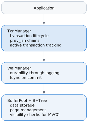
The Transaction Manager is the coordinator - it doesn't store data itself, but ensures that all operations follow ACID rules by orchestrating the WAL, tracking state, and enforcing invariants.
Checkpointing
The Problem
Without checkpointing, two bad things happen:
- WAL grows forever - Every transaction appends records, file gets huge
- Recovery takes forever - After crash, must replay entire WAL from the beginning
After a year of operation the WAL holds millions of records stretching back to day one, and recovery has to replay every one of them. Without checkpoints, startup time grows without bound.
The Solution
A checkpoint says: "Everything up to this point is safely on disk in the main database file. We don't need the old WAL records anymore."
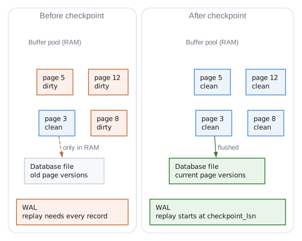
How It Works Step by Step
Step 1: Write CHECKPOINT_BEGIN to WAL
WAL: [...existing records...][CHECKPOINT_BEGIN, lsn=1000]
This marks the start of the checkpoint. If we crash during checkpointing, recovery sees this and knows a checkpoint was in progress.
Step 2: Sync WAL
fsync(wal_file)
Ensures CHECKPOINT_BEGIN is on disk before we start flushing pages.
Step 3: Flush Dirty Pages
Scan the buffer pool and write dirty pages to the database file:
for each frame in buffer_pool:
if frame.dirty:
write frame.data to database_file at page offset
frame.dirty = false
Passive mode: Skip pages that are currently pinned (in use by transactions). This avoids blocking active work.
Full mode: Wait for latches if needed. Guarantees all dirty pages are flushed.
Step 4: Sync Database File
fsync(database_file)
Critical! This ensures all the page writes are actually on disk, not sitting in OS buffers.
Step 5: Write CHECKPOINT_END to WAL
WAL: [...][CHECKPOINT_BEGIN][CHECKPOINT_END, lsn=1002]
This marks successful completion. The payload includes stats (pages flushed).
Step 6: Update checkpoint_lsn
wal_header.checkpoint_lsn = 1002 // LSN of CHECKPOINT_END
fsync(wal_file)
This is the key marker for recovery. It says "everything before LSN 1002 is safely on disk."
The Checkpoint Modes
Passive Mode
"Checkpoint what you can without disrupting active work"
for each frame:
if dirty AND not pinned AND can get latch immediately:
flush it
else:
skip it (maybe next time)
Good for: Background checkpointing during normal operation. Doesn't block transactions.
Bad: May leave some dirty pages unflushed.
Full Mode
"Checkpoint everything, wait if necessary"
for each frame:
if dirty:
wait for latch (spin until available)
flush it
Good for: Complete checkpoint before shutdown, or when WAL is getting too large.
Bad: May briefly block transactions waiting for latches.
Truncate Mode
"Full checkpoint, then reset WAL to beginning"
1. Do full checkpoint
2. Truncate WAL file to just the header
3. Reset frame_count to 0
Good for: Reclaiming disk space when WAL has grown large.
Requires: No active readers (they might be reading old WAL frames).
Why CHECKPOINT_BEGIN and CHECKPOINT_END?
Consider what happens if we crash during checkpointing:
| Scenario | What is in the WAL | State of the database file | What recovery does |
|---|---|---|---|
Crash after CHECKPOINT_BEGIN, before any flush | BEGIN with no END | Unchanged | Sees the incomplete checkpoint, ignores it, replays from the previous checkpoint_lsn |
Crash after some flushes, before CHECKPOINT_END | BEGIN with no END | Some pages updated, some not | Sees the incomplete checkpoint and replays from the previous checkpoint_lsn; replay overwrites the partially flushed pages with correct data |
Crash after CHECKPOINT_END | BEGIN and END | Fully flushed | Sees a complete checkpoint and replays from the new checkpoint_lsn |
All three are safe. The checkpoint is only honoured once CHECKPOINT_END is on disk,
so a torn checkpoint costs replay time but never correctness.
Statistics
Each checkpoint returns stats:
CheckpointStats{
pages_flushed: 42, // How many dirty pages written
duration_ns: 15_000_000, // 15ms
checkpoint_lsn: 1002, // New checkpoint position
wal_truncated: false, // Whether WAL was reset
}
Useful for monitoring:
- If
pages_flushedis always high, consider checkpointing more often - If
duration_nsis high, disk might be slow - Track
checkpoint_lsngrowth over time
When to Checkpoint
// Check if WAL has grown too large
if checkpointer.shouldCheckpoint(max_wal_frames: 1000) {
try checkpointer.checkpoint(.passive);
}
Common strategies:
- Size-based: When WAL exceeds N frames
- Time-based: Every N minutes
- Transaction-based: After N commits
- On shutdown: Always do full checkpoint before closing
Integration
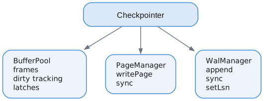
The Checkpointer coordinates between:
- BufferPool: Knows which pages are dirty
- PageManager: Writes pages to database file
- WalManager: Records checkpoint markers, updates checkpoint_lsn
API
var checkpointer = Checkpointer.init(allocator, &bp, &pm, &wal);
// Passive checkpoint (background)
const stats = try checkpointer.checkpoint(.passive);
// Full checkpoint (before shutdown)
const stats = try checkpointer.checkpoint(.full);
// Truncate checkpoint (reclaim WAL space)
const stats = try checkpointer.checkpoint(.truncate);
// Check if checkpoint needed
if (checkpointer.shouldCheckpoint(1000)) {
_ = try checkpointer.checkpoint(.passive);
}
// Get last checkpoint stats
if (checkpointer.getLastStats()) |stats| {
log("Flushed {} pages in {}ms", stats.pages_flushed, stats.duration_ns / 1_000_000);
}
Summary
| Concept | Purpose |
|---|---|
| Dirty page flush | Write modified pages to database file |
| checkpoint_lsn | Recovery starting point |
| CHECKPOINT_BEGIN/END | Crash safety during checkpoint |
| Passive mode | Non-blocking background checkpoint |
| Full mode | Complete checkpoint, may block briefly |
| Truncate mode | Reclaim WAL disk space |
Checkpointing is the bridge between WAL-based durability (fast commits) and bounded recovery time (fast restart). Without it, durability requires replaying the entire history on every startup.
Crash Recovery
The Problem
Databases crash. Power fails, operating systems panic, processes get killed. When this happens, the database must be able to restart and return to a consistent state without losing committed data.
Consider what might be in-flight when a crash occurs:
Scenario: Crash during normal operation
Buffer Pool (RAM):
Page 5: dirty, modified by committed txn
Page 8: dirty, modified by uncommitted txn
Page 12: dirty, partially written by in-progress txn
WAL (Disk):
[committed txn records][uncommitted txn records][partial frame?]
Database File (Disk):
[old versions of pages - some stale, some current]
After restart, we need to:
- Redo committed work - If a transaction committed (COMMIT record in WAL) but its changes weren't flushed to the database file, redo them
- Ignore uncommitted work - If a transaction never committed, pretend it never happened
The ARIES Philosophy
Our recovery is inspired by ARIES (Algorithms for Recovery and Isolation Exploiting Semantics), a recovery algorithm developed at IBM. The key insight:
Write-Ahead Logging + Redo at Recovery = Durability
The WAL contains everything we need. After a crash:
- Read the WAL from the last checkpoint
- Determine which transactions committed
- Redo only committed operations
Two-Phase Recovery
Phase 1: Analysis
Scan the WAL to understand what happened:
| LSN | Record | Transaction | Meaning |
|---|---|---|---|
| 1 | TXN_BEGIN | 1 | Transaction 1 started |
| 2 | INSERT | 1 | Transaction 1 modified data |
| 3 | TXN_BEGIN | 2 | Transaction 2 started |
| 4 | INSERT | 2 | Transaction 2 modified data |
| 5 | TXN_COMMIT | 1 | Transaction 1 committed |
| 6 | UPDATE | 2 | Transaction 2 modified data |
The process crashes after LSN 6, giving:
| Transaction | State |
|---|---|
| 1 | COMMITTED — has TXN_COMMIT |
| 2 | IN_PROGRESS — no commit or abort |
During analysis, we build:
- Transaction table: State of each transaction (committed, aborted, in-progress)
- Redo list: All data operations that might need to be redone
Phase 2: Redo
Apply committed operations to the database:
For each operation in the redo list:
- Check whether its transaction committed. If not, skip it — the change is discarded.
- Apply the operation to the database file.
- Continue to the next operation.
Against the log above:
| LSN | Operation | Transaction | Outcome |
|---|---|---|---|
| 2 | INSERT | 1 | Redo — transaction 1 committed |
| 4 | INSERT | 2 | Skip — transaction 2 never committed |
| 6 | UPDATE | 2 | Skip — transaction 2 never committed |
Why No Undo?
Traditional ARIES has three phases: Analysis, Redo, Undo. We skip Undo because of how we structure our system:
Our approach: Don't apply changes to data pages until commit
- During a transaction, changes are in the buffer pool (RAM)
- On commit, dirty pages are flushed
- On crash, uncommitted changes in RAM are simply lost
Traditional approach: Apply changes immediately, undo on abort
- Changes written to data pages as transaction runs
- If abort/crash, must read WAL backwards and undo each change
- More complex, but allows larger transactions (not limited by RAM)
For an embedded database like Lattice, the simpler "don't undo" approach works well.
The Checkpoint Starting Point
Recovery doesn't scan the entire WAL - only from the last checkpoint:

The checkpoint_lsn in the WAL header marks where recovery begins. The Checkpointer sets this after successfully flushing all dirty pages.
Transaction States
During recovery, each transaction can be in one of three states:
| State | Meaning | WAL Record | Action |
|---|---|---|---|
committed | Completed successfully | TXN_COMMIT present | Redo operations |
aborted | Explicitly rolled back | TXN_ABORT present | Ignore operations |
in_progress | Crash during execution | No commit/abort | Ignore operations |
The distinction between aborted and in_progress is informational - both are handled the same way (ignore their changes).
Record Type Handling
Different WAL records are handled differently:
switch (record.record_type) {
.txn_begin => {
// Track new transaction as in_progress
},
.txn_commit => {
// Mark transaction as committed
},
.txn_abort => {
// Mark transaction as aborted
},
.insert, .update, .delete => {
// Data modification - save for redo phase
},
.page_write => {
// Physical page write - save for redo phase
},
.checkpoint_begin, .checkpoint_end => {
// Informational - no action needed
},
.savepoint, .savepoint_rollback => {
// Track but no special handling
},
.clr => {
// Compensation Log Record - for undo operations
},
}
Physical vs Logical Redo
Our recovery supports two types of operations:
Physical: page_write
Contains the complete page image:
Payload: [page_id: 4 bytes][page_data: 4096 bytes]
Redo: Write entire page directly to database file
Logical: insert, update, delete
Contains the operation parameters:
Payload: [key][value][metadata]
Redo: Re-execute the operation against the B+Tree
For simplicity, our implementation currently relies on page_write for physical durability, with logical operations tracked for statistics.
Corruption Detection
When recovery encounters a checksum mismatch, it must determine whether this is:
- Tail corruption - A torn write at the end of the WAL (safe to proceed)
- Mid-log corruption - Real corruption with valid data after it (unsafe)
Scan-Ahead Detection
On checksum mismatch, we scan ahead to check for valid frames:
Scenario 1 — tail corruption (a torn write)
| Frame | Checksum |
|---|---|
| 0 | OK |
| 1 | OK |
| 2 | Mismatch |
| 3 | Nothing valid |
| 4 | Nothing valid |
No valid frames follow the corruption, so this is a torn write at the end of the WAL. Recovery proceeds with frames 0 and 1.
Scenario 2 — mid-log corruption (real corruption)
| Frame | Checksum |
|---|---|
| 0 | OK |
| 1 | Mismatch |
| 2 | OK |
| 3 | OK |
Valid frames exist after the corrupt one, so this cannot be a torn tail. Recovery
fails with MidLogCorruption rather than silently discarding committed data.
Why This Matters
Mid-log corruption is dangerous because the corrupted frame might contain:
- A
TXN_COMMITrecord we can't see - Data modifications needed for consistency
If we skip the corrupted frame and continue, we might:
- Treat a committed transaction as uncommitted (data loss)
- Apply partial transaction state (inconsistency)
By failing on mid-log corruption, we force manual intervention (restore from backup) rather than silently losing data.
Implementation
fn hasValidFramesAfter(wal: *WalManager, corrupted_frame: u64) bool {
// Check up to 10 frames ahead
for (corrupted_frame + 1 .. min(corrupted_frame + 10, frame_count)) |frame_num| {
if (frameHasValidChecksum(frame_num)) {
return true; // Mid-log corruption!
}
}
return false; // Tail corruption, safe to stop
}
Statistics
Recovery returns detailed statistics:
RecoveryStats{
start_lsn: 1000, // Where we started (checkpoint_lsn)
end_lsn: 1523, // Last valid record
records_scanned: 523, // Total records processed
transactions_found: 15, // Distinct transactions
transactions_committed: 12, // Successfully committed
transactions_aborted: 2, // Explicitly aborted
transactions_rolled_back: 1, // In-progress at crash
redo_operations: 156, // Operations redone
duration_ns: 45_000_000, // 45ms
stopped_at_corruption: true, // Hit tail corruption
corrupted_frame: 42, // Frame number with bad checksum
}
These are useful for:
- Monitoring recovery time
- Debugging transaction issues
- Capacity planning
- Detecting disk health issues (frequent tail corruption may indicate hardware problems)
Recovery Flow Diagram
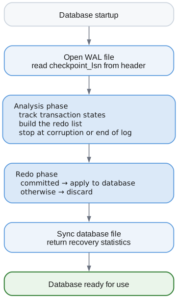
API
// Simple recovery on startup
const stats = try recoverDatabase(allocator, &wal, &pm);
std.debug.print("Recovered {} transactions, redid {} operations in {}ms\n", .{
stats.transactions_committed,
stats.redo_operations,
stats.duration_ns / 1_000_000,
});
// Or use RecoveryManager directly for more control
var rm = RecoveryManager.init(allocator);
const stats = try rm.recover(&wal, &pm);
Integration with Startup
Typical database startup sequence:
1. Open database file (PageManager)
2. Open WAL file (WalManager)
3. Check if recovery needed (WAL has records past checkpoint?)
4. Run recovery
5. Checkpoint to clean slate
6. Ready for operations
Summary
| Concept | Purpose |
|---|---|
| Analysis phase | Determine transaction outcomes |
| Redo phase | Apply committed operations |
| checkpoint_lsn | Recovery starting point |
| Transaction states | committed, aborted, in_progress |
| Checksum verification | Detect corruption/partial writes |
| Tail corruption | Torn write at end, safe to tolerate |
| Mid-log corruption | Real corruption, fail to prevent data loss |
| Scan-ahead detection | Distinguish tail from mid-log corruption |
| No Undo | Uncommitted changes not written to pages |
Recovery transforms a potentially inconsistent crash state into a consistent database by leveraging the WAL as the authoritative record of committed transactions.
Graph Storage
The Property Graph Model
Lattice implements a Labeled Property Graph - the same model used by Neo4j, Amazon Neptune, and other graph databases. It consists of:
Node:
- id: unique identifier (u64)
- labels: set of strings (e.g., "Person", "Employee")
- properties: key-value pairs (e.g., name: "Alice", age: 30)
Edge:
- id: stable unique identifier (u64)
- source: node id
- target: node id
- type: string (e.g., "KNOWS", "WORKS_AT")
- properties: key-value pairs (e.g., since: 2020)
This model is expressive enough to represent almost any domain while remaining simple to query and traverse.
The Storage Challenge
How do you store a graph in a B+Tree (which is fundamentally a key-value store)?
The key insight: decompose the graph into multiple B+Trees, each optimized for a specific access pattern.
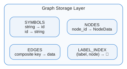
String Interning (Symbol Table)
Graphs have lots of repeated strings: label names, property keys, edge types. Storing "Person" thousands of times wastes space. Instead, we intern strings.
| Interned string | Symbol ID |
|---|---|
"Person" | 1000 |
"Employee" | 1001 |
"name" | 1002 |
"KNOWS" | 1003 |
Storing "Person" costs 6 bytes every time it appears; storing the symbol 1000
costs 2. On a graph with millions of nodes carrying a handful of labels each, that
is most of the property storage.
The Symbol Table uses two B+Trees:
SYMBOLS (forward): SYMBOLS_REVERSE:
"Person" → 1000 1000 → "Person"
"Employee" → 1001 1001 → "Employee"
"name" → 1002 1002 → "name"
"KNOWS" → 1003 1003 → "KNOWS"
Symbol IDs are u16 (0-65535):
- 0: Reserved (null)
- 1-999: Reserved for system use
- 1000-65535: User-defined symbols
API
var symbols = SymbolTable.init(allocator, &forward_tree, &reverse_tree);
// Intern a string (creates if not exists, returns existing if present)
const person_id = try symbols.intern("Person"); // 1000
// Lookup without creating
const id = try symbols.lookup("Person"); // 1000
// or
try symbols.lookup("Unknown"); // SymbolError.NotFound
// Resolve ID back to string
const name = try symbols.resolve(person_id); // "Person"
defer symbols.freeString(name); // Must free allocated string
Node Storage
Nodes are stored in a B+Tree with simple u64 keys:
NODES B+Tree:
Key: node_id (u64, little-endian)
Value: NodeData (serialized)
NodeData Format
NodeData
| Field | Type | Notes |
|---|---|---|
num_labels | u16 | |
labels | u16 × num_labels | Interned symbol ids |
num_properties | u16 | |
properties | PropertyEntry × num_properties |
PropertyEntry
| Field | Type | Notes |
|---|---|---|
key_id | u16 | Interned string id |
value_type | u8 | See the table below |
value_data | variable | Encoding depends on value_type |
Value types
| Code | Type | Encoding |
|---|---|---|
| 0 | Null | No payload |
| 1 | Bool | 1 byte, 0 or 1 |
| 2 | Int64 | 8 bytes, little-endian |
| 3 | Float64 | 8 bytes, IEEE 754 |
| 4 | String | u32 length, then bytes |
| 5 | Bytes | u32 length, then bytes |
| 6 | Vector | u32 length, then f32 values |
| 7 | List | u32 length, then nested values |
| 8 | Map | u32 length, then key/value entries |
Node records are serialized into heap buffers sized from the exact labels and properties being written. The old fixed 4 KiB serialization buffer is no longer part of the node path; large string and bytes properties are handed to the B+Tree, which stores them inline or through overflow pages according to the entry-size rules in B+Tree.
API
var store = NodeStore.init(allocator, &nodes_tree);
// Create a node
const labels = [_]SymbolId{ person_id, employee_id };
const properties = [_]Property{
.{ .key_id = name_id, .value = .{ .string_val = "Alice" } },
.{ .key_id = age_id, .value = .{ .int_val = 30 } },
};
const node_id = try store.create(&labels, &properties);
// Get a node
var node = try store.get(node_id);
defer node.deinit(allocator);
// Check existence
if (store.exists(node_id)) { ... }
// Update a node
try store.update(node_id, &new_labels, &new_properties);
// Delete a node
try store.delete(node_id);
Edge Storage
Edges are more complex because we need efficient traversal in both directions and stable identity for properties, recovery, and parallel edges:
- "Find all people Alice knows" (outgoing)
- "Find all people who know Alice" (incoming)
- "Set this edge's properties after creation" (stable edge ID)
Traversal Tree Plus Edge-ID Index
For edge (Alice)-[:KNOWS]->(Bob), the traversal tree stores two keys and
the payload is stored once in an edge-ID index:
Entry 1 (Outgoing from Alice):
Key: (Alice, OUTGOING, KNOWS, Bob, edge_id)
Value: empty
Entry 2 (Incoming to Bob):
Key: (Bob, INCOMING, KNOWS, Alice, edge_id)
Value: empty
Payload entry:
Key: edge_id
Value: serialized source, target, type, and properties
This keeps traversal efficient in either direction without duplicating large
edge properties. The stable edge_id lets callers update properties by ID and
lets the storage layer restore or delete the exact edge during WAL recovery.
Key Format
Edge keys are 27 bytes, stored big-endian so that byte order matches sort order
and a prefix scan on source_id returns all edges out of a node.
| Offset | Size | Field |
|---|---|---|
| 0–7 | 8 B | source_id: u64 |
| 8 | 1 B | direction: u8 |
| 9–10 | 2 B | type_id: u16 — interned edge type |
| 11–18 | 8 B | target_id: u64 |
| 19–26 | 8 B | edge_id: u64 |
direction | Meaning |
|---|---|
| 0 | Outgoing — source → target |
| 1 | Incoming — target ← source |
Big-endian encoding ensures keys sort correctly for range scans:
- All edges from node X are contiguous
- Within that, all outgoing edges are together
- Within that, edges of same type are together
- Within a source/type/target tuple, parallel edges remain distinct by edge ID
Why This Key Order?
The key (source, direction, type, target) is optimized for common queries:
Query: "All outgoing edges from Alice"
Scan: (Alice, 0, *, *)
Keys are contiguous!
Query: "All KNOWS edges from Alice"
Scan: (Alice, 0, KNOWS, *)
Even more specific prefix!
Query: "Does Alice know Bob?"
Prefix scan: (Alice, 0, KNOWS, Bob, *)
Returns the first matching edge ID, if present
Large edge properties use the same heap serialization and B+Tree overflow path
as node properties. The store checks whether the serialized edge payload can be
represented before replacing an existing edge-ID entry, so oversized updates
return ValueTooLarge without deleting the previous edge record.
API
var store = EdgeStore.init(allocator, &edges_tree, &edge_id_tree);
// Create an edge
const properties = [_]Property{
.{ .key_id = since_id, .value = .{ .int_val = 2020 } },
};
const edge_id = try store.createAndGetId(alice_id, bob_id, knows_id, &properties);
// Get an edge
var edge = try store.get(alice_id, bob_id, knows_id);
defer edge.deinit(allocator);
// Check existence
if (store.exists(alice_id, bob_id, knows_id)) { ... }
// Delete an edge (removes both outgoing and incoming entries)
try store.delete(alice_id, bob_id, knows_id);
// Iterate all outgoing edges from a node
var iter = try store.getOutgoing(alice_id);
defer iter.deinit();
while (try iter.next()) |edge| {
defer edge.deinit(allocator);
// Process edge...
}
// Iterate incoming edges
var incoming = try store.getIncoming(bob_id);
defer incoming.deinit();
// Filter by edge type
var knows_edges = try store.getOutgoingByType(alice_id, knows_id);
defer knows_edges.deinit();
// Count edges without allocating
const out_count = try store.countOutgoing(alice_id);
const in_count = try store.countIncoming(bob_id);
// Property updates use the stable edge ID through the database layer
try db.setEdgePropertyById(null, edge_id, "since", .{ .int_val = 2020 });
Label Index
For queries like MATCH (n:Person), we need to find all nodes with a given label efficiently. The Label Index provides this.
LABEL_INDEX B+Tree:
Key: (label_id: u16, node_id: u64) - big-endian
Value: empty (existence only)
How It Works
When creating node Alice with labels [Person, Employee]:
Insert: (Person, Alice) → ∅
Insert: (Employee, Alice) → ∅
Query "all Person nodes":
Range scan: (Person, 0) to (Person, MAX)
Returns: Alice, Bob, Carol, ...
API
var index = LabelIndex.init(allocator, &label_tree);
// Add labels when creating a node
try index.addLabels(&[_]SymbolId{ person_id, employee_id }, node_id);
// Check if node has a label
if (index.hasLabel(person_id, node_id)) { ... }
// Remove a label from a node
try index.remove(person_id, node_id);
// Get all nodes with a label (allocates result slice)
const person_nodes = try index.getNodesByLabel(person_id);
defer allocator.free(person_nodes);
for (person_nodes) |node_id| {
// Process each Person node...
}
// Lazy iteration (memory-efficient for large result sets)
var iter = try index.iterNodesByLabel(person_id);
defer iter.deinit();
while (try iter.next()) |node_id| {
// Process one node at a time...
}
// Count nodes without allocating
const person_count = try index.countNodesByLabel(person_id);
Putting It Together
A complete graph operation involves multiple B+Trees:
Creating node Alice:Person with name="Alice":
1. Symbol Table:
- intern("Person") → 1000
- intern("name") → 1001
2. Node Store:
- Allocate node_id = 1
- Serialize: [1 label: 1000][1 prop: 1001="Alice"]
- Insert: 1 → serialized_data
3. Label Index:
- Insert: (1000, 1) → ∅
Creating edge (Alice)-[:KNOWS]->(Bob):
1. Symbol Table:
- intern("KNOWS") → 1002
2. Edge Store:
- Allocate edge_id = 1
- Insert traversal keys: (1, OUT, 1002, 2, 1) → ∅ and (2, IN, 1002, 1, 1) → ∅
- Insert payload: 1 → serialized edge data and properties
Performance Characteristics
| Operation | Complexity | Notes |
|---|---|---|
| Create node | O(log n) | One B+Tree insert + label index inserts |
| Get node | O(log n) | Single B+Tree lookup |
| Delete node | O(log n) | One B+Tree delete |
| Create edge | O(log n) | Two traversal inserts + one edge-ID payload insert |
| Get edge | O(log n + k) | Prefix scan to edge ID, then payload lookup |
| Delete edge | O(log n) | Two traversal deletes + one edge-ID payload delete |
| Check label | O(log n) | Single B+Tree lookup |
| Remove label | O(log n) | Single B+Tree delete |
| All nodes with label | O(log n + k) | Range scan, k = result count |
| All edges from node | O(log n + k) | Range scan, k = edge count |
Where n = total items in the respective B+Tree.
Current Limitations
The public database API is not yet fully transaction-isolated end-to-end. The transaction manager contains snapshot-oriented MVCC machinery above this layer, but this chapter only describes the underlying graph-storage structures.
- Property updates rewrite records: No in-place partial property update at the storage-record level
Future Enhancements
- Edge type index: Fast lookup by edge type across all nodes
- Cross-node edge type scans: Dedicated indexes for type-wide traversals
Summary
| Component | B+Tree Key | Purpose |
|---|---|---|
| Symbol Table (forward) | string | String → ID mapping |
| Symbol Table (reverse) | symbol_id | ID → String mapping |
| Node Store | node_id | Node data storage |
| Edge Store | (src, dir, type, tgt, edge_id) | Traversal keys |
| Edge ID Index | edge_id | Stable edge identity and property payload |
| Label Index | (label_id, node_id) | Label-based queries |
| Property Index Catalog | (entity_kind, scope_id, property_id) | Durable explicit index definitions |
| Node Property Index | (scope_id, property_id, value_digest, node_id) | Indexed node-property equality lookup |
| Edge Property Index | (scope_id, property_id, value_digest, edge_id) | Indexed edge-property equality lookup |
The graph storage layer transforms B+Trees into a full property graph database through careful key design, stable edge IDs, and a traversal/payload split for edges.
Vector Search
Overview
Lattice provides approximate nearest neighbor (ANN) search using the HNSW (Hierarchical Navigable Small World) algorithm. This enables semantic search over high-dimensional embedding vectors—a core requirement for AI/RAG applications.
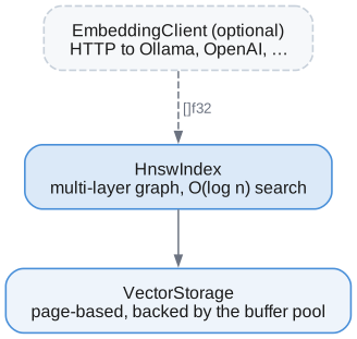
Embedding Generation
Lattice uses a bring your own embeddings approach by default. You can:
- Generate embeddings externally and pass them directly
- Use the optional
EmbeddingClientto call HTTP embedding APIs
Option 1: Bring Your Own Embeddings
// You generate embeddings however you want
const embedding: []const f32 = your_embedding_function("Hello world");
// Insert directly into HNSW index
try hnsw_index.insert(doc_id, embedding);
Option 2: HTTP Embedding Client
The EmbeddingClient calls external HTTP endpoints to generate embeddings. It's disabled by default—you must explicitly create and configure it.
const lattice = @import("lattice");
// Ollama (local) - simplest config
var client = lattice.EmbeddingClient.init(allocator, .{
.endpoint = "http://localhost:11434/api/embeddings",
});
defer client.deinit();
// Generate embedding
const vector = try client.embed("Hello, world!");
defer allocator.free(vector);
Configuration Options
const config = lattice.EmbeddingConfig{
// Required: HTTP endpoint URL
.endpoint = "http://localhost:11434/api/embeddings",
// Model name (default: "nomic-embed-text")
.model = "nomic-embed-text",
// API format: .ollama (default) or .openai
.api_format = .ollama,
// Optional API key for authenticated endpoints
.api_key = null,
// Request timeout in milliseconds (default: 30000)
.timeout_ms = 30_000,
};
Supported API Formats
| Format | Request | Response |
|---|---|---|
.ollama | {"model": "...", "prompt": "..."} | {"embedding": [...]} |
.openai | {"model": "...", "input": "..."} | {"data": [{"embedding": [...]}]} |
Examples
Ollama (local)
var client = EmbeddingClient.init(allocator, .{
.endpoint = "http://localhost:11434/api/embeddings",
.model = "nomic-embed-text",
});
OpenAI
var client = EmbeddingClient.init(allocator, .{
.endpoint = "https://api.openai.com/v1/embeddings",
.model = "text-embedding-3-small",
.api_format = .openai,
.api_key = "sk-...",
});
Local OpenAI-compatible (llama.cpp, vLLM, etc.)
var client = EmbeddingClient.init(allocator, .{
.endpoint = "http://localhost:8080/v1/embeddings",
.model = "local-model",
.api_format = .openai,
});
HNSW Index
HNSW (Hierarchical Navigable Small World) is a graph-based algorithm for approximate nearest neighbor search. It achieves O(log n) search complexity with high recall.
How HNSW Works
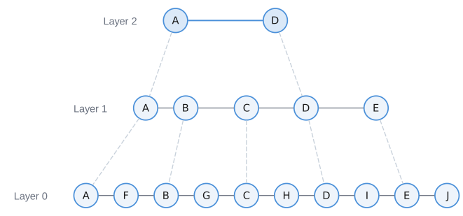
- Upper layers have exponentially fewer nodes (sparse)
- Search starts at top layer, greedily descends
- Layer 0 uses beam search for final candidates
- Each node maintains bidirectional connections to neighbors
Configuration
const config = lattice.HnswConfig{
.m = 16, // Connections per node (layers 1+)
.m_max0 = 32, // Connections at layer 0
.ef_construction = 200, // Search width during insert
.ef_search = 64, // Search width during query
.ml = 0.36067977, // Level multiplier (1/ln(2))
.metric = .cosine, // Distance metric
};
| Parameter | Default | Description |
|---|---|---|
m | 16 | Max connections per node (higher = better recall, more memory) |
m_max0 | 32 | Max connections at layer 0 (typically 2×m) |
ef_construction | 200 | Beam width during insert (higher = better graph quality) |
ef_search | 64 | Beam width during search (higher = better recall, slower) |
metric | .cosine | Distance metric: .euclidean, .cosine, .inner_product |
API Usage
const lattice = @import("lattice");
// Initialize vector storage
var vector_storage = try lattice.VectorStorage.init(allocator, buffer_pool, 384);
defer vector_storage.deinit();
// Initialize HNSW index
var hnsw = lattice.HnswIndex.init(allocator, buffer_pool, &vector_storage, .{
.metric = .cosine,
.ef_search = 100,
});
defer hnsw.deinit();
// Insert vectors
try hnsw.insert(1, embedding1);
try hnsw.insert(2, embedding2);
try hnsw.insert(3, embedding3);
// Search for 10 nearest neighbors
const results = try hnsw.search(query_vector, 10, null);
defer hnsw.freeResults(results);
for (results) |result| {
std.debug.print("ID: {}, Distance: {d:.4}\n", .{ result.id, result.distance });
}
Distance Metrics
| Metric | Formula | Best For |
|---|---|---|
.euclidean | √Σ(aᵢ - bᵢ)² | General purpose |
.cosine | 1 - (a·b)/(‖a‖‖b‖) | Text embeddings (normalized) |
.inner_product | -Σ(aᵢ × bᵢ) | When vectors are pre-normalized |
For text embeddings from most models (OpenAI, Cohere, etc.), use .cosine.
Vector Storage
Vectors are stored in pages managed by the buffer pool, separate from the HNSW graph structure.
| Offset | Size | Field |
|---|---|---|
| 0 | 1 B | page_type: u8 = 0x04 (vector data) |
| 1–2 | 2 B | dimensions: u16 |
| 3–4 | 2 B | vector_count: u16 |
| 5–8 | 4 B | next_page: u32 — overflow chain |
| 9–23 | 15 B | Reserved (header is 24 bytes total) |
| 24 → | variable | Slots, one per vector: [vector_id: u64][f32 × dimensions] |
Pages are 4096 bytes, so a page holds (4096 - 24) / (8 + 4 × dimensions) vectors
before spilling into the next page in the overflow chain.
Vectors per page depends on dimensions:
- 384-dim (1536 bytes): 2 vectors/page
- 768-dim (3072 bytes): 1 vector/page
- 1536-dim (6144 bytes): spans multiple pages
Performance Characteristics
| Operation | Complexity | Notes |
|---|---|---|
| Insert | O(log n) | Builds graph connections |
| Search (k-NN) | O(log n) | Independent of k for small k |
| Delete | O(m × log n) | Removes connections |
| Memory | O(n × m × layers) | ~1KB per vector at m=16 |
Tuning Guidelines
For higher recall:
- Increase
ef_search(e.g., 100-200) - Increase
m(e.g., 32-64) - Use more
ef_construction(e.g., 400)
For faster search:
- Decrease
ef_search(e.g., 32) - Accept lower recall
Typical configuration for 1M vectors:
.m = 16,
.m_max0 = 32,
.ef_construction = 200,
.ef_search = 64, // Adjust based on recall/speed tradeoff
Complete Example
const std = @import("std");
const lattice = @import("lattice");
pub fn main() !void {
var gpa = std.heap.GeneralPurposeAllocator(.{}){};
defer _ = gpa.deinit();
const allocator = gpa.allocator();
// Setup storage (abbreviated)
var buffer_pool = try lattice.BufferPool.init(allocator, page_manager, 1000);
defer buffer_pool.deinit();
// Initialize embedding client (optional)
var embedder = lattice.EmbeddingClient.init(allocator, .{
.endpoint = "http://localhost:11434/api/embeddings",
});
defer embedder.deinit();
// Initialize vector storage and HNSW index
var vector_storage = try lattice.VectorStorage.init(allocator, &buffer_pool, 384);
defer vector_storage.deinit();
var hnsw = lattice.HnswIndex.init(allocator, &buffer_pool, &vector_storage, .{
.metric = .cosine,
});
defer hnsw.deinit();
// Index some documents
const docs = [_][]const u8{
"Zig is a systems programming language",
"Rust focuses on memory safety",
"Go emphasizes simplicity and concurrency",
};
for (docs, 0..) |doc, i| {
const embedding = try embedder.embed(doc);
defer allocator.free(embedding);
try hnsw.insert(i, embedding);
}
// Search
const query_embedding = try embedder.embed("memory safe language");
defer allocator.free(query_embedding);
const results = try hnsw.search(query_embedding, 3, null);
defer hnsw.freeResults(results);
for (results) |result| {
std.debug.print("Doc {}: distance {d:.4}\n", .{ result.id, result.distance });
}
}
SIMD-Optimized Distance Functions
Distance calculations use Zig's @Vector for portable SIMD acceleration. This provides 4-8x speedup over scalar implementations for typical embedding dimensions (384, 768, 1536).
// All distance functions are SIMD-optimized
const dist = lattice.vector.distance.euclideanDistance(vec_a, vec_b);
const cos_dist = lattice.vector.distance.cosineDistance(vec_a, vec_b);
const ip_dist = lattice.vector.distance.innerProductDistance(vec_a, vec_b);
// Additional utilities
const dot = lattice.vector.distance.dotProduct(vec_a, vec_b);
const magnitude = lattice.vector.distance.norm(vec);
lattice.vector.distance.normalize(vec); // in-place
Implementation details:
- Processes 8 floats at a time (AVX-256 compatible)
- Handles non-aligned remainder with scalar fallback
- Works on ARM NEON (128-bit, processed as 2×4)
Current Limitations
- In-memory graph: Node connections stored in memory (persisted to pages on write)
- No incremental persistence: Full graph rebuild on restart
- Single-threaded: No concurrent insert/search yet
Future Enhancements
- Persistent graph: Load HNSW structure from disk
- Concurrent access: Reader-writer locks for parallel search
- Product quantization: Compress vectors for larger datasets
- Filtered search: Combine with label/property predicates
Full-Text Search (BM25)
This document explains how Lattice's full-text search works, from text input to ranked results.
Overview
Full-text search allows you to find documents containing specific words or phrases, ranked by relevance. Lattice implements the BM25 (Best Match 25) ranking algorithm, the same algorithm used by Elasticsearch and other production search engines.
An index covers exactly one label and one property — Document.body, say. You
declare it once, and writing that property keeps it current. Sections 13 to 16
cover how a declaration is stored, how one set of trees carries many indexes, how
writes maintain them, and why the one-label-one-property shape is what lets a
query read the index instead of scanning.
The FTS system consists of five components:

1. Tokenizer
The tokenizer breaks text into searchable tokens.
What It Does
Given input text:
"The quick brown fox jumps over the lazy dog"
The tokenizer produces:
["quick", "brown", "fox", "jumps", "lazy", "dog"]
Notice "The", "the", and "over" are missing—they're stop words.
How It Works
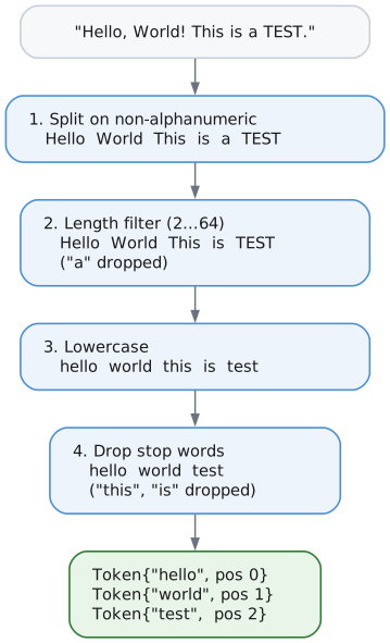
Stop Words
Stop words are common words that add little search value. Lattice supports stop word filtering for 11 languages:
| Language | Example Stop Words |
|---|---|
| English | the, and, is, a, to, of, in, that, it |
| German | der, die, das, und, ist, in, zu, den |
| French | le, la, les, de, et, en, que, un |
| Spanish | el, la, los, de, en, que, y, es |
| Italian | il, la, lo, i, di, e, che, un |
| Portuguese | o, a, os, de, e, que, em, um |
| Dutch | de, het, een, en, van, in, is |
| Swedish | och, i, att, det, en, som, av |
| Norwegian | og, i, det, er, en, at, til |
| Danish | og, i, at, det, en, er, til |
| Finnish | ja, on, ei, ole, oli, se, han |
| Russian | и, в, не, на, что, он, с, как |
Set the language in your tokenizer config:
var tokenizer = Tokenizer.init(allocator, text, .{
.remove_stop_words = true,
.language = .german, // Use German stop words
});
Configuration
pub const TokenizerConfig = struct {
min_token_length: u8 = 2, // Skip tokens shorter than this
max_token_length: u8 = 64, // Skip tokens longer than this
lowercase: bool = true, // Convert to lowercase
remove_accents: bool = true, // Remove diacritics (planned)
remove_stop_words: bool = true, // Filter common words
use_stemming: bool = false, // Apply Porter stemmer
language: Language = .english, // Language for stop words
};
Porter Stemmer
When use_stemming is enabled, tokens are reduced to their root forms:
| Input token | Stemmed |
|---|---|
running | run |
connected | connect |
optimization | optim |
databases | databas |
Why stem? Stemming improves recall by matching morphological variants:
- Query "run" matches documents containing "running", "runs", "runner"
- Query "connect" matches "connected", "connecting", "connection"
Note: Currently only English stemming is supported. For other languages, words are returned unchanged when stemming is enabled. Future versions may add Snowball stemmers for additional languages.
Use normalizeAndStem() or normalizeAndStemWithLanguage() for manual stemming:
var buf: [64]u8 = undefined;
// English stemming
const en_stemmed = tokenizer_mod.normalizeAndStemWithLanguage("RUNNING", &buf, true, .english);
// en_stemmed = "run"
// German (no stemmer available, returns lowercased)
const de_stemmed = tokenizer_mod.normalizeAndStemWithLanguage("RUNNING", &buf, true, .german);
// de_stemmed = "running"
2. Dictionary
The dictionary maps tokens to integer IDs and tracks statistics.
What It Does
| Token | TokenId | DocFreq | PostingPage |
|---|---|---|---|
hello | 1 | 5 | 42 |
world | 2 | 3 | 43 |
database | 3 | 12 | 44 |
search | 4 | 8 | 45 |
Why TokenIds?
Storing the full token string everywhere would waste space. Instead:
- Dictionary stores:
"database"→TokenId 3 - Posting lists store:
TokenId 3(4 bytes instead of 8) - Reduced I/O and memory usage
Storage Format
The dictionary uses a B+Tree with:
- Key: Token string (e.g.,
"hello") - Value: DictionaryEntry (24 bytes)
| Field | Size | Offset |
|---|---|---|
total_freq | 8 B | 0 |
token_id | 4 B | 8 |
doc_freq | 4 B | 12 |
posting_page | 4 B | 16 |
_padding | 4 B | 20 |
Fields are ordered largest-first to minimize internal padding (u64 requires 8-byte alignment).
| Field | Type | Description |
|---|---|---|
total_freq | u64 | Total occurrences across all documents |
token_id | u32 | Unique identifier (1 to ~4 billion) |
doc_freq | u32 | Number of documents containing this token |
posting_page | PageId | First page of the posting list |
_padding | u32 | Explicit padding for 8-byte struct alignment |
Operations
getOrCreate(token) - Get existing TokenId or create new one:
- Look up
"hello"in the B+Tree. - If found, return the existing
token_id. - If not found:
- Assign the next
token_id— say 5. - Insert the token into the B+Tree.
- Return 5.
- Assign the next
3. Posting Lists
A posting list stores which documents contain a specific token.
What It Does
For the token "database" (TokenId 3):
| DocId | TermFreq | |
|---|---|---|
| 15 | 3 | document 15 contains database three times |
| 42 | 1 | |
| 89 | 7 | |
| 156 | 2 | |
| 203 | 1 | |
| … | … |
Page Layout
Each posting list page is 4096 bytes:
| Region | Size | Contents |
|---|---|---|
PageHeader | 8 B | page_type = FTS_POSTING |
PostingPageHeader | 20 B | see below |
| Skip pointers | 16 B each, optional | [doc_id, byte_offset, entry_count] × N |
| Posting data | variable, varint encoded | [doc_id: varint][term_freq: varint] repeated |
PostingPageHeader fields
| Field | Type | Meaning |
|---|---|---|
token_id | u32 | Which token this list belongs to |
num_entries | u32 | Postings held in this page |
next_page | u32 | Overflow page, 0 for none |
num_skip_ptrs | u16 | Number of skip pointers |
flags | u16 | 0x01 = positions present |
data_start | u32 | Byte offset where posting data begins |
PostingPageHeader Explained
The PostingPageHeader is metadata at the start of each posting page:
| Field | Bytes | Purpose |
|---|---|---|
token_id | 4 | Identifies which token this posting list belongs to |
num_entries | 4 | How many (doc_id, term_freq) pairs are in this page |
next_page | 4 | PageId of overflow page if list doesn't fit (0 = no overflow) |
num_skip_pointers | 2 | Count of skip pointers for fast seeking |
flags | 2 | Bit flags: 0x01 = positions stored for phrase queries |
data_start | 4 | Byte offset where posting entries begin (after skip pointers) |
Varint Encoding
Document IDs and frequencies are stored using variable-length integers (varints) for compression:
| Value | Varint bytes | Encoded size | Fixed-width size |
|---|---|---|---|
| 127 | [0x7F] | 1 B | 8 B |
| 128 | [0x80, 0x01] | 2 B | 8 B |
| 16,383 | [0xFF, 0x7F] | 2 B | 8 B |
| 1,000,000 | [0xC0, 0x84, 0x3D] | 3 B | 8 B |
Encoding algorithm:
while value >= 0x80:
output byte = (value & 0x7F) | 0x80 // Low 7 bits + continuation flag
value = value >> 7
output byte = value // Final byte (no continuation)
Example: Encoding 300 (binary: 1 0010 1100)
300 = 0b100101100
Step 1: 300 >= 128, so:
output[0] = (300 & 0x7F) | 0x80 = 0x2C | 0x80 = 0xAC
300 >> 7 = 2
Step 2: 2 < 128, so:
output[1] = 2 = 0x02
Result: [0xAC, 0x02] (2 bytes instead of 8)
Overflow Pages
When a posting list exceeds one page, it chains to overflow pages:
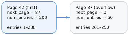
Skip Pointers
Skip pointers enable O(log n) seeking within posting lists, dramatically speeding up multi-term AND queries.
Structure:
| Field | Size | Offset |
|---|---|---|
doc_id | 8 B | 0 |
byte_offset | 4 B | 8 |
entry_count | 4 B | 12 |
How they work:
Skip pointers are created every 128 entries (SKIP_INTERVAL). They record:
doc_id: The document ID at that entrybyte_offset: Where to jump in the posting dataentry_count: Number of entries before this pointer
Posting list with 500 entries:
Skip Pointers:
[0] doc_id=1280, offset=512, count=128 ← entry 128
[1] doc_id=2560, offset=1024, count=256 ← entry 256
[2] doc_id=3840, offset=1536, count=384 ← entry 384
Seeking to doc_id 3000:
1. Binary search skip pointers: find [1] (doc_id=2560 < 3000)
2. Jump to offset 1024
3. Linear scan from entry 256 to find doc_id 3000
Result: Skipped 256 entries instead of scanning all 300
Multi-term intersection optimization:
For AND queries like "database optimization":
- Sort terms by doc_freq (smallest first)
- Iterate through smallest posting list
- For each doc_id, use
skipTo()on other lists - Skip pointers let large lists jump ahead efficiently
Query: "the database" (AND)
"the": 10,000 documents
"database": 100 documents ← Driver (smallest)
Without skip pointers: 10,000 + 100 = 10,100 iterations
With skip pointers: 100 + ~100 seeks = ~200 operations
4. Document Length Storage
BM25 scoring requires knowing each document's length. This is stored in a separate B+Tree:
| DocId | Length (tokens) |
|---|---|
| 1 | 150 |
| 2 | 45 |
| 3 | 892 |
| … | … |
Why store lengths?
BM25 penalizes long documents to prevent them from dominating results just because they contain more words. A 10,000-word document mentioning "database" once is less relevant than a 100-word document mentioning it once.
Statistics tracked:
total_docs: Total documents indexedtotal_tokens: Sum of all document lengthsavg_doc_length: Average tokens per document (for normalization)
5. BM25 Scoring
BM25 calculates a relevance score for each document.
The Formula
Score(D, Q) = Σ IDF(term) × TF_norm(term, D)
for each term in query Q
Where:
IDF (Inverse Document Frequency):
IDF(term) = log((N - df + 0.5) / (df + 0.5) + 1)
N = total number of documents
df = number of documents containing this term
Rare terms get higher IDF scores. If "quantum" appears in 5 of 10,000 documents, it's more significant than "the" appearing in 9,500.
TF_norm (Normalized Term Frequency):
TF_norm = (tf × (k1 + 1)) / (tf + k1 × (1 - b + b × (dl / avgdl)))
tf = term frequency in this document
k1 = saturation parameter (default 1.2)
b = length normalization (default 0.75)
dl = document length
avgdl = average document length
Parameters
| Parameter | Default | Effect |
|---|---|---|
k1 | 1.2 | Controls term frequency saturation. Higher = more weight to repeated terms |
b | 0.75 | Length normalization. 0 = no normalization, 1 = full normalization |
Scoring Example
Corpus: 1000 documents, average length 200 tokens
Query: "database optimization"
Document 42:
- Length: 150 tokens
- "database" appears 3 times
- "optimization" appears 1 time
Term: "database"
- doc_freq = 50 (appears in 50 docs)
- IDF = log((1000 - 50 + 0.5) / (50 + 0.5) + 1) = log(19.82) ≈ 2.99
- tf = 3
- dl/avgdl = 150/200 = 0.75
- TF_norm = (3 × 2.2) / (3 + 1.2 × (1 - 0.75 + 0.75 × 0.75))
= 6.6 / (3 + 1.2 × 0.8125)
= 6.6 / 3.975
≈ 1.66
- Score for "database" = 2.99 × 1.66 ≈ 4.96
Term: "optimization"
- doc_freq = 10 (rarer term)
- IDF = log((1000 - 10 + 0.5) / (10 + 0.5) + 1) ≈ 4.55
- tf = 1
- TF_norm = (1 × 2.2) / (1 + 1.2 × 0.8125) ≈ 1.12
- Score for "optimization" = 4.55 × 1.12 ≈ 5.10
Total Score for Document 42 = 4.96 + 5.10 = 10.06
6. Search Flow
Single-Term Search
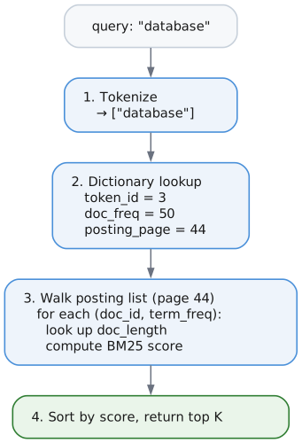
Multi-Term Search (AND Semantics)
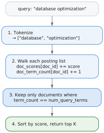
OR Search
OR search returns documents matching any query term:
// Returns docs containing "mysql" OR "postgres" OR both
const results = try fts.searchOr("mysql postgres", 10);
// Or use explicit mode selection
const results = try fts.searchWithMode("mysql postgres", .@"or", 10);
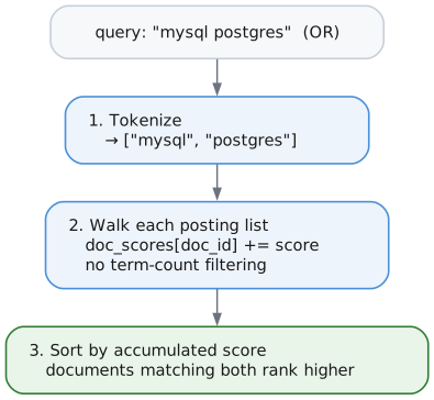
NOT Search (Exclusions)
Prefix terms with - to exclude documents containing them:
// Find "database" docs that don't mention "mysql"
const results = try fts.searchWithMode("database -mysql", .@"and", 10);
// Multiple exclusions
const results = try fts.searchWithMode("database -mysql -oracle", .@"and", 10);
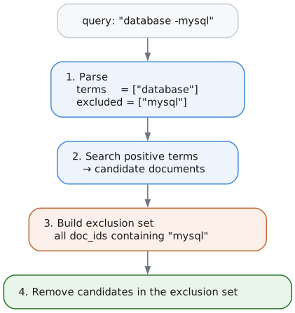
Phrase Search
Phrase search finds documents where terms appear adjacent and in order:
// Enable position storage in config
var fts = FtsIndex.init(allocator, &bp, &dict_tree, &lengths_tree, .{
.store_positions = true,
});
// Search for exact phrase
const results = try fts.searchPhrase("quick brown fox", 10);
Query: "quick brown fox" (phrase)
Document 1: "The quick brown fox jumps" ← MATCHES (adjacent: pos 1,2,3)
Document 2: "A quick red brown fox" ← NO MATCH (not adjacent)
Document 3: "The brown quick fox" ← NO MATCH (wrong order)
How it works:
-
Fetch the posting lists with positions:
Term Postings quickdoc 1 @ 1, doc 2 @ 1 browndoc 1 @ 2, doc 2 @ 3 foxdoc 1 @ 3, doc 2 @ 4 -
For each candidate document, check that the positions are adjacent:
Document Positions Adjacent? doc 1 quick@1,brown@2,fox@3Yes — 1+1=2 and 1+2=3, so it matches doc 2 quick@1,brown@3,fox@4No — 1+1=2 but brownis at 3
Note: Phrase queries require store_positions = true in FtsConfig. Without positions, searchPhrase() falls back to AND semantics.
Quoted Phrase Syntax
You can also use quoted strings in regular search() and searchWithMode() calls to automatically detect phrase queries:
// These are equivalent:
const results1 = try fts.searchPhrase("quick brown", 10);
const results2 = try fts.searchWithMode("\"quick brown\"", .@"and", 10);
Combining phrases with terms and exclusions:
// Phrase + additional term (AND mode)
// Matches documents with "quick brown" phrase AND term "jumps"
const results = try fts.searchWithMode("\"quick brown\" jumps", .@"and", 10);
// Phrase + exclusion
// Matches documents with "quick brown" phrase but NOT containing "fox"
const results = try fts.searchWithMode("\"quick brown\" -fox", .@"and", 10);
// Multiple phrases
// Matches documents with both phrases
const results = try fts.searchWithMode("\"quick brown\" \"lazy dog\"", .@"and", 10);
// Phrase with OR mode
// Matches documents with "quick brown" phrase OR term "rabbit"
const results = try fts.searchWithMode("\"quick brown\" rabbit", .@"or", 10);
Single-word quotes:
Single words in quotes are treated as regular terms (since a one-word phrase is just a term):
// These are equivalent:
const results1 = try fts.search("database", 10);
const results2 = try fts.searchWithMode("\"database\"", .@"and", 10);
Fuzzy Search
Fuzzy search finds documents even when query terms contain typos. It uses Levenshtein (edit) distance to match terms within a configurable threshold.
const fuzzy = @import("fts/fuzzy.zig");
// Search with typo tolerance (max 2 edits)
const results = try fts.searchFuzzy("databse", .{
.max_distance = 2, // Allow up to 2 edits
.min_term_length = 4, // Only fuzzy-match terms >= 4 chars
}, 10);
defer fts.freeResults(results);
// Matches documents containing "database" (edit distance 1)
How it works:
Query: "databse" (typo)
↓
Scan dictionary for terms within edit distance 2:
- "database" (distance=1) ✓
- "datastore" (distance=3) ✗
↓
Search matching terms with distance penalty:
- Score("database") × penalty(1) = Score × 0.75
↓
Return ranked results
Distance penalty formula:
penalty = 1.0 - (distance / max_distance)²
Examples (max_distance = 2):
- distance 0: 1.00 (exact match)
- distance 1: 0.75 (25% penalty)
- distance 2: 0.00 (filtered out)
Levenshtein distance counts the minimum single-character edits needed:
- Insertion: "helo" → "hello" (distance 1)
- Deletion: "hello" → "helo" (distance 1)
- Substitution: "hello" → "hallo" (distance 1)
Note: Transpositions ("recieve" → "receive") count as 2 edits in standard Levenshtein.
Prefix/Wildcard Search
Prefix search finds documents containing terms that start with a given prefix. Use * as a suffix wildcard.
const prefix = @import("fts/prefix.zig");
// Search for terms starting with "optim" (matches "optimize", "optimization", "optimizer")
const results = try fts.searchWithPrefix("optim*", .{
.min_prefix_length = 2, // Minimum prefix length (prevents "a*" explosion)
.max_expansions = 50, // Maximum terms to expand
}, 10);
defer fts.freeResults(results);
How it works:
Query: "optim*"
↓
Calculate range bounds: ["optim", "optin")
↓
B+Tree range scan to find matching terms:
- "optimization" ✓
- "optimize" ✓
- "optimizer" ✓
↓
Search all matching terms (like OR query)
↓
Return ranked results
Combining prefix with regular terms:
// AND semantics: documents must contain "systems" AND a term starting with "data"
const results = try fts.searchWithPrefix("systems data*", .{}, 10);
// Matches documents with both "systems" and "database"/"datastore"/"data"
Constraints:
- Suffix wildcards only (
optim*), not prefix wildcards (*tion) - No middle wildcards (
da*base) - Minimum prefix length configurable (default 2 chars)
- Maximum expansions capped to prevent explosion
Search Highlighting
Search highlighting returns text snippets with matched terms marked, enabling UI display of search results with context.
const highlight = @import("fts/highlight.zig");
const text = "The database stores data efficiently for optimal performance.";
const query_terms = [_][]const u8{ "database", "data" };
const result = try highlight.highlight(
allocator,
text,
&query_terms,
.{ .use_stemming = false }, // TokenizerConfig
.{
.context_chars = 80, // Characters of context around matches
.max_snippets = 3, // Maximum snippets to return
.merge_distance = 40, // Merge snippets closer than this
.prefix_marker = "<em>", // Marker before matched terms
.suffix_marker = "</em>", // Marker after matched terms
.ellipsis = "...", // Added when text is truncated
},
);
defer highlight.freeResult(allocator, result);
// result.snippets[0].text = "The <em>database</em> stores <em>data</em> efficiently..."
// result.total_matches = 2
How it works:
Query terms: ["database", "data"]
Document: "The database stores data efficiently for optimal performance."
↓
Re-tokenize document with same config:
- "database" at offset 4 → stems to "databas" or "database"
- "data" at offset 20 → stems to "data"
↓
Match against query terms (stemmed comparison):
- Match found at positions 4-12 and 20-24
↓
Group matches into snippets with context:
- Single snippet with both matches (close together)
↓
Insert markers around matches:
- "The <em>database</em> stores <em>data</em> efficiently..."
With stemming:
const text = "The runners were running fast in the marathon.";
const query_terms = [_][]const u8{"run"}; // Already stemmed query
const result = try highlight.highlight(
allocator,
text,
&query_terms,
.{ .use_stemming = true }, // Enable stemming
.{ .prefix_marker = "**", .suffix_marker = "**" },
);
// "running" stems to "run" → match
// "runners" stems to "runner" → no match
// result.snippets[0].text = "The runners were **running** fast..."
Key design decisions:
- Re-tokenization approach: Document text is re-tokenized at query time (no storage overhead)
- Stemmed matching: Query terms are matched against stemmed document tokens
- Original text preserved: Markers wrap the original text, not stemmed forms
- Configurable markers: Default
<em>/</em>but customizable for any format - Snippet merging: Close matches combined into single snippets
Finding matches only (without snippets):
const matches = try highlight.findMatches(
allocator,
text,
&query_terms,
.{ .use_stemming = false },
);
defer highlight.freeMatches(allocator, matches);
for (matches) |match| {
// match.start = byte offset of match start
// match.end = byte offset of match end (exclusive)
const matched_text = text[match.start..match.end];
}
7. Indexing Flow
Nothing calls this directly any more. Writing an indexed property is what runs it, and section 15 covers how that happens. The mechanics below are unchanged: this is what one document costs whenever it is indexed.
Indexing one document
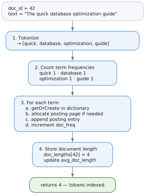
8. Data Structures Summary
In-Memory
| Structure | Purpose |
|---|---|
Tokenizer | Streaming text tokenization |
PostingIterator | Iterate posting list entries |
Bm25Scorer | Calculate relevance scores |
On-Disk (B+Trees)
| B+Tree | Key | Value |
|---|---|---|
| Dictionary | 4-byte scope prefix + token string | DictionaryEntry (24 bytes) |
| DocLengths | 4-byte scope prefix + DocId (8 bytes) | Length (4 bytes) |
| Reverse index | 4-byte scope prefix + DocId | Terms the document contributed |
| Index catalog | [kind, scope_id, property_id] | empty; the key is the record |
The scope prefix is what keeps one declared index out of another's way; section 14 explains it. The catalog shares its tree with the property indexes, under different kind discriminators.
On-Disk (Pages)
| Page Type | Content |
|---|---|
FTS_POSTING | Posting list entries (varint encoded) |
9. Limitations and Future Work
Current Limitations
- English-only stemming - Porter stemmer for English only (other languages skip stemming)
- One property per index - Searching several fields as one document means storing the combined text in a property and indexing that. The reasoning is in the design note: an index spanning
titleandbodywould maked.title @@ "x"match on body text, which is the confusion per-property indexes exist to remove. - Selectivity is per term, not per phrase - the estimate that chooses between two indexes is the rarest term's document frequency, which bounds an AND query correctly but says nothing about how often the terms occur together. Two predicates whose terms are individually common but jointly rare estimate as common.
- Fuzzy matching does not reach uncommitted text - Text written in the current transaction is matched by term presence rather than edit distance, because fuzzy expansion walks the committed dictionary.
Implemented Features
- Phrase queries -
searchPhrase("quick brown fox")with position verification - Boolean queries - AND (default), OR (
searchOr), NOT (-termsyntax) - Porter stemming -
use_stemming=truereduces words to roots (English) - Position indexing -
store_positions=truefor phrase queries - Skip pointers - O(log n) posting list intersection for multi-term queries
- Quoted phrase syntax - Parse
"exact phrase"in regular search() calls - Fuzzy search - Levenshtein distance for typo tolerance via
searchFuzzy() - Multi-language stop words - 11 languages supported (EN, DE, FR, ES, IT, PT, NL, SV, NO, DA, FI, RU)
- Prefix/wildcard search -
searchWithPrefix("optim*")expands to matching terms - Search highlighting -
highlight()returns snippets with matched terms marked - Document deletion -
removeDocument()with reverse index properly cleans posting lists and stats - Per-property indexes - one index per label and property, declared and then maintained by writes (sections 13 to 15)
- Relationship indexes - the same over a relationship type and property
- Index seek as the access path - a full-text predicate reads the index instead of filtering a label scan (section 16)
- Corpus statistics on disk - document count and average length survive a reopen, so scores do not depend on what the session happened to index
Planned Features
- Multi-language stemmers - Snowball stemmers for German, French, etc.
10. The Index Component Directly
This is the engine component, wired up by hand. It is here to show what the
pieces above do together, not as an API to use: nothing outside the storage layer
constructs an FtsIndex, and indexDocument is reached by writing an indexed
property rather than by calling it.
For the API you would actually use, see Full-Text Search (@@) and the full-text search guide.
const std = @import("std");
const lattice = @import("lattice");
pub fn main() !void {
var gpa = std.heap.DebugAllocator(.{}){};
const allocator = gpa.allocator();
// Initialize storage (simplified)
var bp = try BufferPool.init(allocator, &pm, 64 * 4096);
var dict_tree = try BTree.init(allocator, &bp);
var lengths_tree = try BTree.init(allocator, &bp);
// Create FTS index with phrase query support
var fts = FtsIndex.init(allocator, &bp, &dict_tree, &lengths_tree, .{
.store_positions = true, // Enable phrase queries
});
// Index documents
_ = try fts.indexDocument(1, "Introduction to database systems");
_ = try fts.indexDocument(2, "Advanced database optimization techniques");
_ = try fts.indexDocument(3, "Web development with JavaScript");
_ = try fts.indexDocument(4, "Database performance and MySQL tuning");
// Basic AND search (all terms must match)
const results1 = try fts.search("database optimization", 10);
defer fts.freeResults(results1);
// Returns doc 2 (contains both terms)
// OR search (any term matches)
const results2 = try fts.searchOr("mysql postgres", 10);
defer fts.freeResults(results2);
// Returns doc 4 (contains "mysql")
// NOT search (exclusions with -prefix)
const results3 = try fts.searchWithMode("database -mysql", .@"and", 10);
defer fts.freeResults(results3);
// Returns docs 1, 2 (contain "database" but not "mysql")
// Phrase search (exact sequence)
const results4 = try fts.searchPhrase("database systems", 10);
defer fts.freeResults(results4);
// Returns doc 1 (has "database systems" as adjacent phrase)
// Quoted phrase syntax (alternative to searchPhrase)
// Phrase "database optimization" + term "advanced"
const results5 = try fts.searchWithMode("\"database optimization\" advanced", .@"and", 10);
defer fts.freeResults(results5);
// Returns doc 2 (has phrase "database optimization" AND term "advanced")
// Fuzzy search (typo tolerance)
const results6 = try fts.searchFuzzy("databse", .{
.max_distance = 2,
.min_term_length = 4,
}, 10);
defer fts.freeResults(results6);
// Returns docs with "database" (edit distance 1 from "databse")
for (results1) |result| {
std.debug.print("Doc {}: score {d:.2}\n", .{ result.doc_id, result.score });
}
}
11. Serialization Pattern
All on-disk structures use extern struct with compile-time size assertions:
/// Good: Self-documenting, compile-time verified
pub const PostingPageHeader = extern struct {
token_id: TokenId,
num_entries: u32,
next_page: PageId,
num_skip_pointers: u16,
flags: u16,
data_start: u32,
comptime {
std.debug.assert(@sizeOf(PostingPageHeader) == 20);
}
pub fn read(data: []const u8) PostingPageHeader {
return std.mem.bytesAsValue(PostingPageHeader, data[OFFSET..][0..@sizeOf(PostingPageHeader)]).*;
}
pub fn write(self: *const PostingPageHeader, data: []u8) void {
@memcpy(data[OFFSET..][0..@sizeOf(PostingPageHeader)], std.mem.asBytes(self));
}
};
Why this pattern?
- No magic numbers - Field layout is defined by the struct, not manual offsets
- Compile-time verification -
comptimeblock catches size mismatches immediately - Self-documenting - Struct fields serve as documentation
- Consistent with codebase - WAL, PageHeader, FileHeader all use this pattern
Alignment considerations:
When structs contain u64 fields, use explicit padding and order fields largest-first:
pub const DictionaryEntry = extern struct {
total_freq: u64, // 8 bytes - largest first (requires 8-byte alignment)
token_id: u32, // 4 bytes
doc_freq: u32, // 4 bytes
posting_page: u32, // 4 bytes
_padding: u32 = 0, // 4 bytes - explicit trailing padding
comptime {
std.debug.assert(@sizeOf(DictionaryEntry) == 24);
}
};
13. Declared Indexes
An index covers one label and one property. Nothing is indexed until you say so.
try db.createNodeFtsIndex("Document", "body");
Declaring reads body from every node already carrying Document and indexes
it, so adding an index to a database full of documents makes them searchable
immediately rather than only affecting what arrives afterwards. That mirrors what
createNodePropertyIndex does, for the same reason: an index that only covers
future writes is a trap.
Where a declaration lives
Declarations go in the same B+Tree as the property index catalog, under their own kind discriminators:
| Kind | Meaning |
|---|---|
| 1 | node property index |
| 2 | edge property index |
| 3 | node full-text index |
| 4 | edge full-text index |
The key is [kind (1 byte), scope_id (2 bytes big-endian), property_id (2 bytes big-endian)] and the value is empty — the key is the whole record. scope_id is
a label for a node index and a relationship type for an edge one; both are symbol
ids from the same table the rest of the engine uses.
Sharing the catalog tree was free. The key already began with a kind byte, so
adding two more kinds needed no format change and no new tree. Big-endian is what
makes a range scan over one kind possible: [3] to [4] covers every node
full-text declaration and nothing else.
Why not multiple properties per index
Storing several properties as one document is easy. Asking for it is not. If an
index merged title and body, then WHERE d.title @@ "x" would match documents
whose body contained the term, and the property name would be lying — which is
the exact confusion per-property indexes exist to remove. Reusing property access
as the query syntax requires one property per index.
Somebody who wants several fields ranked as one document stores the combined text in a property and indexes that. The text is then visible in the database, where it can be read and rebuilt, instead of living only inside an index.
14. One Set of Trees, Many Indexes
Every declared index shares the dictionary, document-length, and reverse-index
trees. Without something separating them, a term indexed for title would be
found by a search of body.
Every key written for an index carries a four-byte prefix naming it:
[kind (1), scope_id (2 BE), property_id (1)] ++ the key the store wanted
So bread in Document.title and bread in Document.body are two different
keys in one tree, and a range over a prefix walks one index's terms and stops.
Why a view rather than a prefix argument
The prefix is applied by a wrapper — ScopedTree — that the stores hold in place
of a raw B+Tree. The stores' key-building code did not change at all.
The alternative was passing a prefix into each place that builds a key, of which there are about a dozen across three files. Missing one would not fail to compile. It would write an entry the matching read could never find, or read another index's entries. One place to get right beats twelve places to remember.
The prefix arithmetic
Walking one index means ranging from its prefix to the next one. Computing "the
next prefix" has a trap: a prefix ending in 0xFF has to carry into the byte
before it. Incrementing the last byte alone wraps to zero, producing an upper
bound below the lower one, and the index reads as empty. That carry is a
function with its cases tested rather than arithmetic written inline twice.
Where the prefix comes off again
Reads strip the prefix before returning keys, because callers want the term. This matters more than it sounds: fuzzy search measures edit distance against the term text, so four bytes of index identity on the front puts every term far outside any sensible distance and nothing ever matches. The stripping lives in the iterator, next to the prefixing, so the two cannot drift apart.
15. Keeping Indexes Current
Writing an indexed property maintains the index. There is no separate indexing call, and nothing to forget.
Create, update, and delete all funnel through one function per entity kind, where an empty old state means a create and an empty new state means a delete. Eight call sites reach those two functions, which is eight fewer places that could each decide what a change means.
What is indexed
Only string properties. A number, a list, or an absent property contributes
nothing. Rendering 42 as "42" so a text search could match it would be a
different feature with different rules, and doing half of it silently would make
results hard to explain.
Unchanged text is left alone
An update whose indexed text did not change skips the index entirely. Without that, writing any property on an entity would reindex its longest indexed string, and the cost of an unrelated write would scale with how much text the entity happens to carry.
Recovery
Redo replays into the stores directly rather than through the write path, so nothing maintains the indexes while it runs — the same situation the property indexes are already in. After a redo, each declared index is cleared and rebuilt.
The clear works by scope prefix rather than by walking documents. An entity the redo deleted is no longer there to walk, so walking would leave its terms behind to keep matching. Deleting by prefix is a batched collect-then-delete, because the tree's iterator pins a leaf and holds a slot in it, which makes deleting during iteration unsafe; a fixed batch keeps memory flat rather than proportional to what is often the largest structure in the database.
Posting pages of a cleared index stay allocated. Nothing points at them once the dictionary entries naming them are gone, so it is wasted space rather than wrong data, and reclaiming it needs page reuse the store does not have yet.
16. Search as an Access Path
A @@ predicate is planned as the way into the data, not as a filter over a scan.
Why per-property indexing is what makes this possible
A Document.body index contains only Document nodes. The index is already
label-scoped, so reading it does the label scan's job and answers the text
question at the same time. The older design — one index spanning every node —
could not have done this: it had no idea which nodes carried which label, so it
could only ever filter a scan somebody else produced.
The measurement
Eight thousand documents, a query matching one of them:
| time | |
|---|---|
| the index lookup alone | 31 µs |
| scanning the label and keeping what the index named | 72 ms |
the same predicate under an AND, filtered per row | 216 ms |
The scan cost the whole corpus to answer a question the index had already answered. Seeking instead:
| before | after | |
|---|---|---|
@@ 'rare' | 72 ms | 105 µs |
@@ 'rare' AND … | 216 ms | 105 µs |
@@ 'common' AND … | 21.3 s | 320 ms |
Selective queries also stopped growing with the corpus — 65 µs, 80 µs, 105 µs from five hundred to eight thousand documents, against 3.9 ms, 17 ms, 72 ms before.
When it applies
Only in conjunctive positions: the whole WHERE, or a branch of an AND.
Under an OR the planner deliberately does not seek. The other branch can admit
entities the index never names, so seeking would silently drop rows. There is a
test asserting that an OR plans a label scan, because the reason is not visible
from reading the planner and the shape looks like a missed optimisation.
The predicate also has to name the entity the pattern is about. Where the variable is already bound by an upstream expand, the input decides which rows exist and the index can only filter them.
The filter that remains
What cannot be sought is still answered by evaluating @@ per row. That path
consults the index once per query rather than once per row, keyed on the
resolved index and the query text, and held for one execution.
Without it the filter was quadratic in the corpus: its cost against a scan grew 8.4x, 22.2x, then 152.1x as the corpus grew, and is now a flat 2.4x, 2.7x, 2.3x.
Reusing a search within one execution is the same assumption the scanning operators have always made — they search once when they open and use that result for every row they emit. The cache matches that granularity rather than inventing a stricter or a looser rule.
Choosing between two ways in
d.title @@ "the" AND d.body @@ "sourdough" offers two ways into the data, and
they are not equally cheap. Starting from a word most documents share means
reading the corpus to discard it; starting from a rare one means reading almost
nothing.
The dictionary already records, for every term, how many documents contain it. An AND query cannot match more documents than its rarest term appears in, so the minimum of those counts is a real upper bound rather than a guess — and a term absent from the dictionary gives zero, which is exact. Each candidate costs one B-tree lookup per term to estimate.
The choice is made when the query runs, not when it is planned, for two reasons. A query whose text arrives as a parameter has nothing to estimate at plan time. And a cached plan would carry a decision made against whatever the data looked like when it was first planned.
Choosing at execution is safe because the filter above the seek applies the whole condition regardless of which candidate was read, so the choice can only affect how much work is done, never which rows come back.
Candidates are confined to one label. The label the access path guarantees is the one whose filter the planner skips, and which candidate runs is not known until it runs; candidates spanning two labels would mean skipping a filter the chosen path does not satisfy. That was a real defect during development — a pattern asking for two labels returned entities carrying only one — and it survived two tests that passed for an unrelated reason before a negative control exposed it.
Measured on eight thousand documents, one matching row:
| query | before | after |
|---|---|---|
| rare predicate written first | 4.3 ms | 4.3 ms |
| common predicate written first | 244 ms | 4.2 ms |
The point is not only the 59x. It is that the two rows now agree: how the author ordered the predicates no longer decides what the query costs.
Disjunctions
Several @@ predicates on one variable joined by OR are planned as a single
operator that reads each index once and unions the results. A document found by
more than one takes its best score rather than a sum: two properties matching is
not evidence that either matched twice as well, and adding them would rank a
document matching both weakly above one matching a single property strongly.
Mixing kinds is refused. d.title @@ "x" OR r.note @@ "x" cannot be one union,
because one operator filters one slot and a slot holds a node or an edge. That
query still answers correctly, through the row filter.
12. File Reference
| File | Purpose |
|---|---|
src/fts/tokenizer.zig | Text tokenization, normalization, language config |
src/fts/stopwords.zig | Multi-language stop word lists (11 languages) |
src/fts/dictionary.zig | Token → TokenId mapping via B+Tree, range iteration |
src/fts/posting.zig | Posting list storage with varint encoding, entry removal |
src/fts/scorer.zig | BM25 scoring, document length storage |
src/fts/index.zig | Main FtsIndex coordinator, boolean/phrase/fuzzy/prefix search |
src/fts/stemmer.zig | Porter stemmer algorithm (English), language routing |
src/fts/fuzzy.zig | Levenshtein distance, fuzzy term expansion |
src/fts/prefix.zig | Prefix/wildcard search, upper bound calculation |
src/fts/highlight.zig | Search result highlighting, snippet extraction |
src/fts/reverse_index.zig | doc_id → terms mapping for document deletion |
src/fts/catalog.zig | Declared indexes: kind, scope, property |
src/fts/scoped_tree.zig | Prefixing view that keeps declared indexes apart |
src/query/operators/fts.zig | Index seek and filtering operators |
Query Execution
Overview
Lattice executes Cypher queries using the Volcano iterator model—a pull-based execution engine where operators form a tree and data flows upward one row at a time. This design enables lazy evaluation, memory efficiency, and composable query plans.
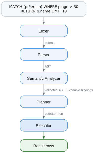
The Volcano Iterator Model
Every operator implements three methods:
pub const Operator = struct {
vtable: *const VTable,
ptr: *anyopaque,
pub const VTable = struct {
open: fn (*anyopaque, *ExecutionContext) OperatorError!void,
next: fn (*anyopaque, *ExecutionContext) OperatorError!?*Row,
close: fn (*anyopaque, *ExecutionContext) void,
deinit: fn (*anyopaque, Allocator) void,
};
};
- open(): Initialize the operator, acquire resources (iterators, memory)
- next(): Return the next row, or
nullif exhausted - close(): Release resources (unpin pages, close iterators)
- deinit(): Free the operator itself
Pull-Based Execution
Data flows upward through the operator tree. The root operator "pulls" from its children:
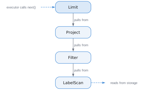
When the executor calls root.next():
- Limit calls Project.next()
- Project calls Filter.next()
- Filter calls LabelScan.next()
- LabelScan reads from B+Tree, returns row
- Filter evaluates predicate—if false, pulls another row
- Project evaluates expressions, transforms row
- Limit checks count, returns row (or null if limit reached)
Lazy Evaluation
Work happens only when next() is called. For LIMIT 10, we might scan millions of nodes but only process 10 matching rows. Unused rows are never materialized.
Rows and Slots
A Row is a fixed-size tuple flowing between operators:
pub const Row = struct {
slots: [16]SlotValue, // Variable bindings
distances: [16]f32, // Vector search distances
scores: [16]f32, // FTS relevance scores
populated: u16, // Bitmask of populated slots
};
Slot Values
Each slot holds one of:
pub const SlotValue = union(enum) {
empty: void, // Unset
node_ref: NodeId, // Reference to a node (just the ID)
edge_ref: EdgeId, // Reference to an edge
property: PropertyValue, // Actual value (int, string, bool, etc.)
};
Why Slots Instead of Named Variables?
Performance. Looking up slots[3] is O(1). The planner assigns each variable to a numbered slot:
| Pattern element | Slot |
|---|---|
(p:Person) | 0 |
[r:KNOWS] | 1 |
(f:Person) | 2 |
The execution context maintains the mapping from names to slots for expression evaluation.
Lazy Materialization
Rows store references (NodeId, EdgeId), not full objects. Properties are fetched on-demand during expression evaluation. This avoids loading data that's never accessed.
Operators
Scan Operators
AllNodesScan: Iterates every node in the database.
open(): Create B+Tree iterator (null start key = first entry)
next(): Read entry, extract NodeId from key, set output slot
close(): Release iterator, unpin pages
LabelScan: Iterates nodes with a specific label.
open(): Create LabelIndex iterator for the label
next(): Get next NodeId from index, set output slot
close(): Release iterator
Both produce rows with a single slot containing a node reference.
Filter Operator
Evaluates a predicate and passes through only matching rows.
fn next(self: *Filter, ctx: *ExecutionContext) !?*Row {
while (true) {
const row = try self.input.next(ctx) orelse return null;
const result = try self.evaluator.evaluate(self.predicate, row, ctx);
if (result.isTruthy()) {
return row;
}
// Predicate failed, try next row
}
}
Supports short-circuit evaluation for AND/OR.
Project Operator
Transforms rows by evaluating expressions for each output column.
| Return item | Expression |
|---|---|
p.name | expr[0] |
p.age + 1 | expr[1] |
"literal" | expr[2] |
fn next(self: *Project, ctx: *ExecutionContext) !?*Row {
const input_row = try self.input.next(ctx) orelse return null;
self.output_row.clear();
for (self.items) |item| {
const value = try self.evaluator.evaluate(item.expr, input_row, ctx);
self.output_row.setSlot(item.output_slot, resultToSlotValue(value));
}
return self.output_row;
}
Expand Operator
Traverses edges from input nodes. This implements pattern matching like (a)-[r]->(b).
State:
source_slot = slot containing the source node
target_slot = slot to write target node
edge_slot = slot to write edge (optional)
edge_iterator = current iterator over edges
current_input = row being expanded
next():
loop:
if edge_iterator.next() returns edge:
output_row = copy input row
output_row[target_slot] = edge.target
output_row[edge_slot] = edge (if requested)
return output_row
// Exhausted edges for current input, get next input
current_input = input.next()
if null: return null
source = current_input[source_slot]
edge_iterator = edgeStore.getOutgoing(source)
This is a one-to-many operator: one input row can produce multiple output rows.
Supports three directions:
outgoing:(a)-[r]->(b)— traverse outgoing edgesincoming:(a)<-[r]-(b)— traverse incoming edgesboth:(a)-[r]-(b)— traverse both directions
Limit and Skip
Limit: Returns at most N rows.
fn next(self: *Limit, ctx: *ExecutionContext) !?*Row {
if (self.returned >= self.count) return null;
const row = try self.input.next(ctx) orelse return null;
self.returned += 1;
return row;
}
Skip: Discards the first N rows.
fn next(self: *Skip, ctx: *ExecutionContext) !?*Row {
while (self.skipped < self.count) {
_ = try self.input.next(ctx) orelse return null;
self.skipped += 1;
}
return try self.input.next(ctx);
}
Sort Operator (Blocking)
Sort must see all input before producing any output—it's a blocking operator.
fn open(self: *Sort, ctx: *ExecutionContext) !void {
try self.input.open(ctx);
// Materialize all input rows
while (try self.input.next(ctx)) |row| {
try self.rows.append(row.*);
}
// Sort in memory
self.sortRows();
}
fn next(self: *Sort, ctx: *ExecutionContext) !?*Row {
if (self.index >= self.rows.items.len) return null;
defer self.index += 1;
return &self.rows.items[self.index];
}
This breaks the streaming model but is necessary for ordering.
Vector Search Operator
Performs k-NN search using the HNSW index.
fn open(self: *VectorSearch, ctx: *ExecutionContext) !void {
// Execute search upfront
self.results = try self.index.search(self.query_vector, self.k, null);
}
fn next(self: *VectorSearch, ctx: *ExecutionContext) !?*Row {
while (self.current < self.results.len) {
const result = self.results[self.current];
self.current += 1;
// Apply distance threshold
if (self.threshold) |t| {
if (result.distance > t) continue;
}
self.row.setSlot(self.output_slot, .{ .node_ref = result.node_id });
self.row.setDistance(self.output_slot, result.distance);
return self.row;
}
return null;
}
The distance is stored in the row for use in expressions or sorting.
FTS Operators
There are two, and which one the planner picks is the difference between reading an index and reading a corpus.
FtsIndexSeek is a leaf. It searches the declared index and emits one row per
hit, in score order. It has no input because it needs none: a Document.body
index holds only Document nodes, so seeking it does the label scan's job as well
as answering the text question.
fn open(self: *FtsIndexSeek, ctx: *ExecutionContext) !void {
self.results = try runSearches(self.database, ctx, self.searches, self.limit, self.allocator);
}
fn next(self: *FtsIndexSeek, _: *ExecutionContext) !?*Row {
const hit = self.results.?[self.current_index];
self.current_index += 1;
self.row.?.setSlot(self.output_slot, .{ .node_ref = hit.doc_id });
self.row.?.setScore(self.output_slot, hit.score);
return self.row;
}
FtsSearchWithInput filters rows somebody else produced, keeping those the index named. It is what runs when the entity is already bound by an upstream expand, so the input decides which rows exist and the index can only narrow them.
Both run their searches through one shared function, so they cannot come to
disagree about what a disjunction of @@ predicates means.
The full reasoning, including the measurements that motivated the seek, is in Full-Text Search, section 16.
Mutation Operators
Mutation operators modify the graph structure. Unlike read operators, they have side effects.
CreateNode: Creates new nodes with labels and properties.
fn next(self: *CreateNode, ctx: *ExecutionContext) !?*Row {
const node_id = try ctx.storage.createNode(self.labels);
for (self.properties) |prop| {
const value = try self.evaluator.evaluate(prop.value, null, ctx);
try ctx.storage.setProperty(node_id, prop.key, value);
}
self.output_row.setSlot(self.output_slot, .{ .node_ref = node_id });
return &self.output_row;
}
DeleteNode: Removes nodes from the graph. With DETACH, also removes connected edges.
fn next(self: *DeleteNode, ctx: *ExecutionContext) !?*Row {
const row = try self.input.next(ctx) orelse return null;
const node_id = row.slots[self.target_slot].node_ref;
if (self.detach) {
try ctx.storage.detachDelete(node_id);
} else {
try ctx.storage.deleteNode(node_id);
}
return row; // Pass through for chaining
}
SetProperty: Updates properties on nodes or edges.
MATCH (n:Person {name: "Alice"}) SET n.age = 31, n.city = "NYC"
fn next(self: *SetProperty, ctx: *ExecutionContext) !?*Row {
const row = try self.input.next(ctx) orelse return null;
const target = row.slots[self.target_slot];
const value = try self.evaluator.evaluate(self.value_expr, row, ctx);
// SET n.prop = NULL removes the property
if (value == .null_val) {
try ctx.storage.removeProperty(target, self.property_name);
} else {
try ctx.storage.setProperty(target, self.property_name, value);
}
return row;
}
SetLabels: Adds labels to nodes.
MATCH (n:Person {name: "Alice"}) SET n:Admin:Verified
RemoveProperty: Explicitly removes properties.
MATCH (n:Person {name: "Alice"}) REMOVE n.city
RemoveLabel: Removes labels from nodes.
MATCH (n:Person {name: "Alice"}) REMOVE n:Verified
Expression Evaluation
The expression evaluator handles predicates and projections.
pub fn evaluate(expr: *const Expression, row: *const Row, ctx: *ExecutionContext) !EvalResult {
return switch (expr.*) {
.literal => |lit| evaluateLiteral(lit),
.variable => |v| evaluateVariable(v, row, ctx),
.property_access => |pa| evaluatePropertyAccess(pa, row, ctx),
.binary => |b| evaluateBinary(b, row, ctx),
.unary => |u| evaluateUnary(u, row, ctx),
.function_call => |f| evaluateFunction(f, row, ctx),
// ...
};
}
Supported Operations
Comparison: =, <>, <, <=, >, >=
Logical: AND, OR, NOT, XOR (with short-circuit evaluation)
Arithmetic: +, -, *, /, %, ^
String: CONTAINS, STARTS WITH, ENDS WITH
Null handling: IS NULL, IS NOT NULL
Functions: id(), coalesce(), abs(), size(), toInteger(), toFloat()
Vector Search: <=> (vector distance operator)
-- k-NN search with distance threshold
MATCH (c:Chunk) WHERE c.embedding <=> $query < 0.5 RETURN c
Full-Text Search: @@ (FTS match operator)
-- BM25-scored full-text search
MATCH (d:Doc) WHERE d.text @@ $search RETURN d
MATCH (d:Doc) WHERE d.text @@ "neural networks" RETURN d
These operators are recognized by the planner and converted to specialized search operators that use the HNSW and FTS indexes directly, rather than scanning all nodes.
For full-text search that holds only in conjunctive positions — the whole WHERE,
or a branch of an AND. Under an OR the planner keeps the label scan on
purpose, because the other branch can admit entities the index never names and
seeking would silently drop them.
Type Coercion
Numeric operations promote integers to floats when mixed:
42 + 3.14 → 45.14 (float)
Null propagates through most operations:
null + 1 → null
null = null → true (special case for equality)
The Query Planner
The planner transforms an AST into an operator tree by walking the query clauses.
Planning Algorithm
pub fn plan(query: *Query) !Operator {
var current: ?Operator = null;
for (query.clauses) |clause| {
current = switch (clause) {
.match => try planMatch(clause.match, current),
.where => try planWhere(clause.where, current),
.create => try planCreate(clause.create, current),
.delete => try planDelete(clause.delete, current),
.set => try planSet(clause.set, current),
.remove => try planRemove(clause.remove, current),
.return_ => try planReturn(clause.return_, current),
.order_by => try planOrderBy(clause.order_by, current),
.limit => try planLimit(clause.limit, current),
.skip => try planSkip(clause.skip, current),
};
}
return current.?;
}
Example: Simple Query
MATCH (p:Person) WHERE p.age > 30 RETURN p.name LIMIT 10
Produces:
Limit(count=10)
└── Project([p.name → slot 0])
└── Filter(p.age > 30)
└── LabelScan(label="Person", output=slot 0)
Example: Edge Traversal
MATCH (a:Person)-[:KNOWS]->(b:Person) RETURN a.name, b.name
Produces:
Project([a.name → slot 0, b.name → slot 1])
└── Expand(source=0, target=1, type="KNOWS", dir=outgoing)
└── LabelScan(label="Person", output=slot 0)
Variable Binding
The planner allocates slots for variables:
| Variable | Slot | Kind |
|---|---|---|
| a | 0 | node |
| b | 1 | node |
| r | 2 | edge |
These bindings are registered in the ExecutionContext for expression evaluation.
Execution Context
Runtime state for query execution:
pub const ExecutionContext = struct {
allocator: Allocator,
row_arena: ArenaAllocator, // Fast row allocation
parameters: StringHashMap(Value), // Query parameters ($name)
variables: StringHashMap(u8), // Variable → slot mapping
};
Row Arena
Rows are allocated from an arena that's reset between queries. This avoids per-row allocation overhead:
// During query execution
const row = try ctx.allocRow(); // Fast bump allocation
// After query completes
ctx.resetRowArena(); // Frees all rows at once
Query Parameters
Parameters allow safe value injection:
MATCH (p:Person) WHERE p.age > $min_age RETURN p
try ctx.setParameter("min_age", .{ .int_val = 30 });
Operator Composition
Operators are composable—any operator can wrap any other:
// Filter wrapping Expand wrapping LabelScan
Filter
└── Expand
└── LabelScan
// Limit wrapping Sort wrapping Filter
Limit
└── Sort
└── Filter
└── ...
This enables flexible query plans without special-casing combinations.
Memory Management
Operator Lifecycle
1. Planner creates operators (heap allocated)
2. Executor calls open() on root (cascades down)
3. Executor calls next() repeatedly (rows flow up)
4. Executor calls close() on root (cascades down)
5. Executor calls deinit() on root (frees operators bottom-up)
Iterator Cleanup
Operators holding B+Tree or index iterators must release them in close():
fn close(self: *LabelScan, ctx: *ExecutionContext) void {
if (self.iterator) |*iter| {
iter.deinit(); // Unpins pages in buffer pool
self.iterator = null;
}
}
Failing to do this leaks pinned pages.
Future Optimizations
The current planner uses simple heuristics. Future improvements could include:
Predicate Pushdown
Move filters closer to scans:
Before: Filter(a.x > 10) → Expand → LabelScan
After: Expand → Filter(a.x > 10) → LabelScan
Cost-Based Index Selection
The planner already selects explicit property indexes for eligible inline and
immediately following WHERE equalities. A future cost model could choose
between available label and property indexes using cardinality and selectivity
statistics instead of the current first-eligible heuristic.
Join Ordering
For multi-pattern queries, order joins by estimated cardinality.
Vectorized Execution
Process rows in batches instead of one-at-a-time for better cache utilization.
Database Query API
The Database.query() method provides the primary interface for executing Cypher queries. It orchestrates all components of the query pipeline.
Basic Usage
// Open database
var db = try Database.open(allocator, "mydb.ltdb", .{ .create = true });
defer db.close();
// Create some data
_ = try db.createNode(&[_][]const u8{"Person"});
_ = try db.createNode(&[_][]const u8{"Person"});
// Execute a query
var result = try db.query("MATCH (n:Person) RETURN n");
defer result.deinit(); // Always clean up results
// Process results
std.debug.print("Found {} rows\n", .{result.rowCount()});
for (result.rows) |row| {
for (row.values) |val| {
switch (val) {
.node_id => |id| std.debug.print("Node: {}\n", .{id}),
.string_val => |s| std.debug.print("String: {s}\n", .{s}),
.int_val => |i| std.debug.print("Int: {}\n", .{i}),
.null_val => std.debug.print("null\n", .{}),
else => {},
}
}
}
Result Types
/// A single value in a query result
pub const ResultValue = union(enum) {
null_val: void, // NULL
bool_val: bool, // true/false
int_val: i64, // integers
float_val: f64, // floating point
string_val: []const u8, // strings
node_id: NodeId, // node reference
};
/// A row in a query result
pub const ResultRow = struct {
values: []ResultValue, // One value per column
};
/// Complete query result
pub const QueryResult = struct {
columns: [][]const u8, // Column names from RETURN clause
rows: []ResultRow, // Result rows
allocator: Allocator,
pub fn deinit(self: *QueryResult) void; // Free all memory
pub fn rowCount(self: *const QueryResult) usize;
pub fn columnCount(self: *const QueryResult) usize;
};
Error Handling
The query() method returns QueryError on failure:
pub const QueryError = error{
ParseError, // Syntax error in Cypher
SemanticError, // Undefined variable, type mismatch
PlanError, // Query cannot be planned
ExecutionError, // Runtime error during execution
OutOfMemory,
};
Example error handling:
const result = db.query("MATCH (n RETURN n"); // Missing )
if (result) |r| {
defer r.deinit();
// process results
} else |err| switch (err) {
QueryError.ParseError => std.debug.print("Syntax error\n", .{}),
QueryError.SemanticError => std.debug.print("Semantic error\n", .{}),
else => std.debug.print("Query failed: {}\n", .{err}),
}
Internal Pipeline
When you call db.query(cypher), the following happens:
1. Parser.init(allocator, cypher)
└── parser.parse() → AST (or ParseError)
2. SemanticAnalyzer.init(allocator)
└── analyzer.analyze(ast) → AnalysisResult (or SemanticError)
3. QueryPlanner.init(allocator, storage_context)
└── planner.plan(ast, analysis) → Operator tree (or PlanError)
4. ExecutionContext.init(allocator)
└── Register variable bindings from planner
5. execute(allocator, root_operator, context)
└── Pull rows through operator tree → executor.QueryResult
6. convertResult(exec_result, planner)
└── Transform to user-friendly QueryResult
The StorageContext connects the planner to database storage:
const storage_ctx = StorageContext{
.node_tree = &self.node_tree, // B+Tree for nodes
.label_index = &self.label_index, // Label → NodeId index
.edge_store = &self.edge_store, // Edge storage
.symbol_table = &self.symbol_table, // String interning
};
Memory Management
- QueryResult owns all memory: Call
deinit()when done - Strings are copied: Safe to use after query components are freed
- Row arena: Internal rows use arena allocation, reset between queries
Files
| File | Purpose |
|---|---|
src/storage/database.zig | Database.query() API, QueryResult types |
src/query/executor.zig | Operator interface, Row, ExecutionContext |
src/query/expression.zig | Expression evaluator |
src/query/planner.zig | AST to operator tree transformation |
src/query/operators/scan.zig | AllNodesScan, LabelScan |
src/query/operators/filter.zig | Filter operator |
src/query/operators/project.zig | Project operator |
src/query/operators/expand.zig | Edge traversal |
src/query/operators/vector.zig | HNSW k-NN search |
src/query/operators/fts.zig | Full-text search |
src/query/operators/limit.zig | Limit, Skip, Sort |
src/query/operators/mutation.zig | CREATE, DELETE, SET, REMOVE |
Benchmarks
Benchmarked on Apple M1, single-threaded, with auto-scaled buffer pool.
Core Operations
| Operation | Latency | Throughput | Target | Status |
|---|---|---|---|---|
| Node lookup | 0.13 us | 7.9M ops/sec | < 1 us | PASS |
| Node creation | 0.65 us | 1.5M ops/sec | — | — |
| Edge traversal | 9 us | 111K ops/sec | — | — |
| Full-text search (100 docs) | 19 us | 53K ops/sec | — | — |
| 10-NN vector search (1M vectors) | 0.83 ms | 1.2K ops/sec | < 10 ms @ 1M | PASS |
Vector Search (HNSW) at Scale
128-dimensional cosine vectors, M=16, ef_construction=200, ef_search=64, k=10.
| Scale | Mean Latency | P99 Latency | Recall@10 | Memory |
|---|---|---|---|---|
| 1,000 | 65 us | 70 us | 100% | 1 MB |
| 10,000 | 174 us | 695 us | 99% | 10 MB |
| 100,000 | 438 us | 1.2 ms | 99% | 101 MB |
| 1,000,000 | 832 us | 1.8 ms | 100% | 1,040 MB |
Search latency scales sub-linearly (O(log N)) with 99-100% recall@10. Uses heuristic neighbor selection (HNSW paper Algorithm 4) for diverse graph connectivity, connection page packing for ~4.5x memory reduction, and pre-normalized dot product for fast cosine distance.
ef_search Sensitivity (1M vectors)
| ef_search | Mean Latency | Recall@10 |
|---|---|---|
| 16 | 506 us | 57% |
| 32 | 1.9 ms | 79% |
| 64 | 990 us | 100% |
| 128 | 3.2 ms | 100% |
| 256 | 11.6 ms | 100% |
Optimization History
Baseline (pre-optimization)
| Scale | Insert Rate | Search Mean | Recall@10 |
|---|---|---|---|
| 1K | ~91/sec | 1.7ms | 100% |
| 10K | ~42/sec | 3.8ms | 99% |
| 100K | ~23/sec | 4.5ms | 99% |
| 1M | ~14/sec | 6.4ms | 100% |
Post-optimization (Phase 2)
Six optimizations applied: last_page tracking, pre-sized search structures, stack-buffer connection I/O, cached vectors in heuristic pruning, pre-normalize + dot product for cosine.
| Scale | Insert Rate | Search Mean | Recall@10 |
|---|---|---|---|
| 1K | ~954/sec | 65us | 100% |
| 10K | ~726/sec | 174us | 99% |
| 100K | ~526/sec | 438us | 99% |
| 1M | ~248/sec | 832us | 100% |
Improvement Summary
| Scale | Insert Speedup | Search Speedup |
|---|---|---|
| 1K | 10.5x | 26x |
| 10K | 17.5x | 22x |
| 100K | 22.8x | 10x |
| 1M | 17.7x | 7.7x |
Reproducing
zig build benchmark # Core operation benchmarks
zig build vector-benchmark -- --quick # Vector benchmarks (1K/10K/100K, ~7 min)
zig build vector-benchmark # Full vector benchmarks including 1M (~70 min)
zig build graph-benchmark -- --quick # Graph traversal benchmarks
Competitive Analysis
Point Lookups
| System | Latency | Type | Source |
|---|---|---|---|
| LatticeDB | 0.13 us | Embedded | zig build benchmark |
| RocksDB (in-memory) | 0.14 us | Embedded | RocksDB wiki |
| SQLite (in-memory) | ~0.2 us | Embedded | Turso blog |
| SQLite (WAL, disk) | 3 us (p90) | Embedded | marending.dev |
| Neo4j | 28 ms (p99) | Server | Memgraph comparison |
LatticeDB's B+Tree achieves sub-microsecond cached lookups, matching RocksDB in-memory and outperforming SQLite on disk by 23x.
Vector Search
| System | Latency (10-NN) | Scale | Type | Source |
|---|---|---|---|---|
| LatticeDB | 0.83 ms mean, 100% recall | 1M | Embedded | zig build vector-benchmark |
| FAISS HNSW (single-thread) | 0.5-3 ms | 1M | Library | FAISS wiki |
| Weaviate | 1.4 ms mean, 3.1 ms P99 | 1M | Server | Weaviate benchmarks |
| Qdrant | ~1-2 ms | 1M | Server | Qdrant benchmarks |
| Milvus + SQ8 | 2.2 ms P99 | 1M | Server | VectorDBBench |
| pgvector HNSW | ~5 ms @ 99% recall | 1M | Extension | Jonathan Katz |
| LanceDB | 3-5 ms | 1M | Embedded | LanceDB blog |
| Chroma | 4-5 ms mean | 1M | Embedded | Chroma docs |
| Pinecone P2 | ~15 ms (incl. network) | 1M | Cloud | Pinecone blog |
| sqlite-vec (brute force) | 17 ms | 1M | Extension | Alex Garcia |
LatticeDB at 1M achieves 0.83 ms mean with 100% recall@10 — faster than FAISS single-threaded HNSW and competitive with Weaviate and Qdrant server-based systems (which add network overhead in practice).
Graph Traversal
| System | 2-hop (100K nodes) | Type | Source |
|---|---|---|---|
| LatticeDB | 39 us | Embedded | zig build sqlite-benchmark |
| SQLite (recursive CTE) | 548 us | Embedded | zig build sqlite-benchmark |
| Kuzu (archived Oct 2025) | 19 ms | Embedded | The Data Quarry |
| Neo4j | 10 ms (1M nodes) | Server | Neo4j blog |
Numbers marked with a third-party source were measured on hardware and with methodology we do not control, and are not directly comparable to the LatticeDB figures. Only the SQLite comparison below is head to head. Kùzu was archived in October 2025 following its creators' acquisition; see vs Kùzu and LadybugDB.
LatticeDB vs SQLite
Social network graph with power-law degree distribution, adjacency cache pre-warmed.
Small Scale (10K nodes, 50K edges)
| Workload | LatticeDB | SQLite | Speedup |
|---|---|---|---|
| 1-hop traversal | 560 ns | 13.0 us | 23x |
| 2-hop traversal | 3.0 us | 37.5 us | 13x |
| 3-hop traversal | 19.1 us | 178.5 us | 9x |
| Variable path (1..5) | 82.4 us | 4.3 ms | 52x |
Medium Scale (100K nodes, 500K edges)
| Workload | LatticeDB | SQLite | Speedup |
|---|---|---|---|
| 1-hop traversal | 8.0 us | 290.0 us | 36x |
| 2-hop traversal | 38.7 us | 548.3 us | 14x |
| 3-hop traversal | 197.3 us | 1.2 ms | 6x |
| Variable path (1..5) | 134.4 us | 10.1 ms | 75x |
Depth-Limited Traversal (10K nodes, 50K edges)
| Depth | LatticeDB | SQLite | Speedup |
|---|---|---|---|
| 10 | 311 us | 121 ms | 390x |
| 15 | 380 us | 271 ms | 713x |
| 25 | 318 us | 587 ms | 1,848x |
| 50 | 500 us | 1.4 s | 2,819x |
LatticeDB uses BFS with adjacency cache and bitset visited tracking. SQLite uses a recursive CTE with UNION deduplication. Both compute identical reachable node sets (~8K nodes). The gap widens at deeper depths as SQLite's CTE overhead grows with each recursion level.
Full-Text Search (BM25)
| System | Search Latency | Type | Source |
|---|---|---|---|
| LatticeDB | 19 us | Embedded | zig build benchmark |
| SQLite FTS5 | < 6 ms | Embedded | SQLite Cloud |
| Elasticsearch | 1-10 ms | Server | Various |
| Tantivy | 10-100 us | Library | Various |
LatticeDB's inverted index with BM25 scoring is ~300x faster than SQLite FTS5 and competitive with Tantivy (a dedicated Rust search library).
Building from Source
LatticeDB is written in Zig with zero external dependencies.
Prerequisites
- Zig 0.16.0 (the version used by CI and release workflows)
Clone and Build
git clone https://github.com/jeffhajewski/latticedb.git
cd latticedb
zig build # build everything
Build Targets
zig build # Build everything
zig build lib # Build static library only
zig build cli # Build CLI tool only
zig build shared # Build shared library for bindings
Optimized Builds
zig build -Doptimize=ReleaseSafe # Release build with safety checks
zig build -Doptimize=ReleaseFast # Optimized release build
Building Language Bindings
Python
# Build the shared library first
zig build shared
# The Python bindings use ctypes to load the shared library
cd bindings/python
pip install -e .
TypeScript
# Build the shared library first
zig build shared
# Build the TypeScript bindings
cd bindings/typescript
npm install
npm run build
Project Structure
src/
├── core/ # Core types and utilities
├── storage/ # B+Tree, page management, WAL
├── vector/ # HNSW index, vector operations
├── fts/ # Full-text search, tokenizer
├── query/ # Cypher parser, planner, executor
├── transaction/ # Transaction management, MVCC
├── concurrency/ # Locking, latches
├── api/ # C API bindings
└── cli/ # CLI tool
include/
└── lattice.h # C API header
bindings/
├── python/ # Python bindings
├── typescript/ # TypeScript/Node.js bindings
└── go/ # Go bindings
Running Tests
LatticeDB has a comprehensive test suite covering unit tests, integration tests, concurrency tests, crash recovery tests, and benchmarks.
Test Commands
zig build test # Run unit tests
zig build integration-test # Run integration tests
zig build crash-test # Run crash recovery tests
zig build shared # Build shared library used by bindings
Benchmarks
zig build benchmark # Core operation benchmarks
zig build vector-benchmark -- --quick # Vector benchmarks (1K/10K/100K, ~7 min)
zig build vector-benchmark # Full vector benchmarks including 1M (~70 min)
zig build graph-benchmark -- --quick # Graph traversal benchmarks
Test Structure
tests/
├── unit/ # Unit tests for individual modules
├── integration/ # End-to-end integration tests
├── fuzz/ # Fuzzing targets for parser and serialization
├── crash/ # Crash recovery tests (kill process mid-transaction)
├── container/ # Linux package/shared-library smoke tests
└── benchmark/ # Performance benchmarks
Testing Standards
- Aim for 100% branch coverage on core modules
- Fuzzing is mandatory for the parser and serialization code
- Crash recovery is tested by killing the process mid-transaction and verifying data integrity
- Concurrency tests cover all multi-threaded code paths
TypeScript Binding Tests
cd bindings/typescript
npm test
Python Binding Tests
cd bindings/python
uv run --extra dev pytest tests -q
Release Checks
Before tagging a release, validate version consistency and the binding smoke paths:
python3 scripts/bump_version.py --check <version> --strict-lockfile
zig build test
zig build integration-test
zig build shared
cd bindings/typescript && npm test -- --runInBand
Releasing
Use scripts/prepare_release.sh as the supported release entry point. It wraps
the repository-wide version bumper, optional lockfile refresh, consistency
checks, tests, and optional tag creation.
Patch Release Flow
scripts/prepare_release.sh 0.9.6
git diff
git status --short --branch
git add build.zig src/main.zig src/api/c_api.zig include/lattice.h bindings/ examples/ conformance/ book/src/api/c.md
git commit -m "Release v0.9.6"
git tag v0.9.6
git push origin main
git push origin v0.9.6
Use --tag or --push-tag when you want the script to create or push the tag
for you:
scripts/prepare_release.sh 0.9.6 --tag
scripts/prepare_release.sh 0.9.6 --tag --push-tag
Version Sources
scripts/bump_version.py is the canonical version updater/checker. It updates
and validates:
- native source and C header versions:
build.zig,src/main.zig,src/api/c_api.zig,include/lattice.h - the Zig package manifest version:
build.zig.zon - Python metadata:
bindings/python/pyproject.toml,bindings/python/src/latticedb/__init__.py,bindings/python/uv.lock - TypeScript metadata and fallback version:
bindings/typescript/package.json,bindings/typescript/package-lock.json,bindings/typescript/src/index.ts - example and conformance dependency pins for Go and TypeScript
- the C API version example in
book/src/api/c.md
Before pushing a release tag, run:
python3 scripts/bump_version.py --check 0.9.6 --strict-lockfile
The GitHub release workflow runs the same strict check before building or publishing artifacts.
Validation
For a normal release, keep the default scripts/prepare_release.sh test run
enabled. For manual validation, use:
zig build test
zig build integration-test
zig build shared
cd bindings/python && uv run --extra dev pytest tests -q
cd bindings/typescript && npm test -- --runInBand
Storage changes that affect durability, page layout, large values, recovery, or bindings should also run the relevant crash, container, or regression repro tests before tagging.
Contributing
Contributions to LatticeDB are welcome.
Getting Started
- Fork the repository on GitHub
- Clone your fork and create a branch
- Make your changes
- Run the test suite:
zig build test - Submit a pull request
Development Setup
git clone https://github.com/YOUR_USERNAME/latticedb.git
cd latticedb
zig build test # Verify everything builds and passes
Code Style
- Follow existing Zig conventions in the codebase
- All allocation goes through explicit allocator parameters
- Fail fast: detect and report corruption, don't hide it
- Keep the C API as the contract: all bindings wrap
include/lattice.h
Testing
All changes should include appropriate tests:
- Unit tests for new functions or modules
- Integration tests for end-to-end behavior changes
- Fuzz tests for parser or serialization changes
- Crash tests for durability-related changes
Run the full test suite before submitting:
zig build test
zig build integration-test
Pull Requests
- Keep PRs focused on a single change
- Include a clear description of what changed and why
- Ensure all tests pass
- Add tests for new functionality
Reporting Issues
File issues on GitHub with:
- A clear description of the problem
- Steps to reproduce
- Expected vs actual behavior
- LatticeDB version and platform